In physics and materials science, local structure means the arrangement of the nearest neighbours around a particular atom in a crystal or molecule: which atoms surround it, how far away they are, and how symmetrically they are arranged. It is the atom's immediate neighbourhood, as opposed to the long-range, repeating pattern of the crystal as a whole.
The distinction matters because real materials are never perfect. A crystal can be highly ordered over long distances while containing impurities, missing atoms, atoms squeezed between regular sites, or small distortions. Many of the properties that make materials useful in electronics, batteries, solar cells and magnetic storage are controlled by exactly these local imperfections. Yet the most familiar structural methods, X-ray and neutron diffraction, average over enormous numbers of atoms, and so they are largely insensitive to what happens around one particular kind of atom.
Nuclear spectroscopy offers a way around that. By using specific atomic nuclei as tiny probes, methods such as nuclear magnetic resonance (NMR), Mössbauer spectroscopy and perturbed angular correlation (PAC) can sense the electric and magnetic fields at a single lattice site, and from those fields infer the local structure. This article explains what local structure is, why diffraction misses it, how the hyperfine interaction makes nuclei into probes, how the main techniques work, what they have been used for, and where their limits lie. It also covers complementary non-nuclear methods, such as X-ray absorption fine structure and pair distribution function analysis, that address the same question from a different angle.
Long-range order and local structure
Crystals as repeating patterns
A crystal is a solid in which atoms are arranged in a pattern that repeats in three dimensions. The smallest repeating block is the unit cell, and the whole crystal can be thought of as many copies of that block stacked together. Crystals can grow very large when conditions are right; the Wikipedia article on local structure cites the giant crystals of the Naica Mine in Mexico as an example of how far that long-range order can extend.
Diffraction methods exploit the repetition. When X-rays or neutrons pass through a crystal, waves scattered from the regularly spaced planes of atoms interfere, producing sharp intensity peaks, called Bragg peaks, at particular angles. From the positions and intensities of those peaks, crystallographers work out the average unit cell: the spacing of the lattice and the average position of each kind of atom within it.
What averaging hides
The word "average" is the key. A diffraction pattern comes from billions of unit cells at once. Suppose that one atom in a thousand is replaced by an impurity, or that some atoms sit slightly off their ideal positions in a random way. The Bragg peaks will hardly change. The defect is real, and may control an important property, but diffraction is, in the words of the Wikipedia article, "insensitive to effects in local structure."
| Feature | Long-range (average) structure | Local structure |
|---|---|---|
| Question answered | What is the repeating pattern of the crystal? | What surrounds this particular atom? |
| Typical method | X-ray or neutron diffraction (Bragg peaks) | Nuclear probes, X-ray absorption fine structure, pair distribution function |
| Sensitive to rare defects? | Weakly | Yes, if the probe sits at or near the defect |
| Length scale | Many unit cells | Nearest neighbours, roughly within 1 nm |
| Example output | Lattice constants, average atomic positions | Neighbour distances, site symmetry, local fields |
Kinds of local disorder
Real crystals contain many kinds of local deviation from the ideal pattern:
- Substitutional impurities: a foreign atom occupies a regular lattice site.
- Interstitial atoms: an atom sits between lattice sites, where no atom should be.
- Vacancies: a lattice site is empty.
- Defect complexes: combinations, such as an impurity bound to a neighbouring vacancy.
- Local distortions: neighbours shift slightly to accommodate a defect, or a material distorts locally even when its average structure looks undistorted.
- Disorder in nanomaterials: in very small particles, a large fraction of atoms sit at or near surfaces, where the environment differs from the interior.
Each of these changes the local structure around nearby atoms, even when it barely affects the average structure.
Why local structure matters
Many functional materials are, in effect, defect materials. Their useful properties are created or controlled by deliberately introduced impurities or by intrinsic defects.
| Application area | Why local structure matters |
|---|---|
| Semiconductors and chips | Dopant atoms placed on specific lattice sites control electrical conductivity; a dopant on the wrong site, or bound to a defect, may not work |
| Solar cells | Defects can trap charge carriers and reduce efficiency |
| Batteries | The local environment of ions affects how easily they move in and out of electrode materials |
| Transparent conducting oxides | Oxides such as indium oxide conduct electricity through defects and dopants |
| Magnetic materials | Local magnetic fields at defects affect the behaviour of magnetic layers in devices |
| Catalysts | Active sites are often local arrangements at surfaces or defects |
The Wikipedia article on local structure highlights functional materials used in electronics, chips, batteries, semiconductors and solar cells, and illustrates the topic with the crystal structure of indium(III) oxide. It also notes the importance of magnetic local structure, the pattern of local magnetic fields in a crystal, for understanding defects in magnetic materials such as those used in giant magnetoresistance (GMR), the effect exploited in hard-disk read heads.
The nucleus as a probe
Scale
The central idea of nuclear local-structure methods is to use the nucleus of an atom as a sensor sitting exactly at the lattice site of interest. The nucleus is extraordinarily small: the Wikipedia article states that it is "about 10,000 to 150,000 times smaller than the atom itself." Because it is so small and sits at the centre of the atom, it experiences the electric and magnetic fields at one point in the crystal rather than an average over a region.
What the nucleus feels
A nucleus is surrounded by its atom's own electrons, and beyond them by neighbouring atoms. Both create electric fields at the nucleus, and if the material is magnetic, there may also be a magnetic field. The interactions between a nucleus and these fields are called hyperfine interactions. They slightly shift and split the energy levels of the nucleus. The name comes from atomic spectroscopy, where hyperfine shifts were seen as an even finer splitting than the "fine structure" caused by electron spin; hyperfine shifts are orders of magnitude smaller than fine-structure shifts.
There are two main hyperfine interactions relevant to local structure.
1. Magnetic dipole interaction. Many nuclei have a magnetic moment. In a magnetic field B at the nucleus, the energy depends on the orientation of the nuclear spin, producing a splitting proportional to the field. Measuring this splitting gives the local magnetic field at the nucleus.
2. Electric quadrupole interaction. Nuclei with spin I ≥ 1 are not perfectly spherical; their charge distribution is slightly elongated or flattened, described by the electric quadrupole moment Q. Such a nucleus does not respond to the electric field itself but to how the field changes across the nucleus, the electric field gradient (EFG).
The electric field gradient
The EFG is defined as the set of second derivatives of the electrostatic potential V at the nucleus, V_ij = ∂²V/∂x_i∂x_j. It forms a symmetric 3 × 3 tensor. When the charges producing it lie outside the nucleus, the tensor is traceless (its diagonal elements sum to zero), so in its principal axes it can be described by just two numbers: the largest component, V_zz, and the asymmetry parameter
η = (V_yy − V_xx) / V_zz, with 0 ≤ η ≤ 1 (the form given in the Wikipedia article on PAC; the sign depends on how the principal axes are labelled).
Three facts about the EFG make it an excellent local-structure probe:
| Property of the EFG | Consequence |
|---|---|
| It is zero for cubic symmetry | Any measurable quadrupole interaction signals that the site's surroundings are not cubic, for example because of a nearby defect |
| It falls off as r⁻³ with distance from the nucleus | It is dominated by the nearest electrons and neighbours, i.e. by local structure |
| In crystals it is of order 10²¹ V/m² | Large enough to produce measurable splittings |
Because of the r⁻³ dependence, the EFG is "highly sensitive to the electronic density in the immediate vicinity of a nucleus," as the Wikipedia article on the EFG puts it. A classic review of the EFG in non-cubic metals by Elton Kaufmann and Reiner Vianden, published in Reviews of Modern Physics in 1979, remains a standard reference for how EFGs arise in metals. Today, density functional theory calculations are routinely used to compute EFGs for candidate structures and compare them with measurements.
From fields to structure
The logic of a nuclear local-structure measurement is therefore indirect but powerful:
- Place a suitable nucleus, the probe, at the site of interest.
- Measure the hyperfine splitting of its energy levels.
- Extract the local magnetic field and/or the EFG (V_zz and η).
- Compare with calculations or reference compounds to identify which local structure produces those values.
A value of η near zero suggests an axially symmetric site; a value near one suggests strong distortion. A change in V_zz when a sample is annealed may reveal that a defect has moved next to the probe. A distribution of values, rather than one sharp value, signals disorder.
The main nuclear techniques
Three nuclear methods are named in the Wikipedia article on local structure: NMR, Mössbauer spectroscopy and PAC. Two related methods, nuclear quadrupole resonance (NQR) and muon spin spectroscopy (μSR), use closely related ideas.
| Technique | What is measured | Typical probe | Needs radioactive source? | Notable strength |
|---|---|---|---|---|
| NMR | Radio-frequency absorption by nuclear spins in a magnetic field | Stable nuclei such as ¹H, ¹³C, quadrupolar nuclei | No | Chemical detail; very widely available |
| NQR | Radio-frequency resonance from the quadrupole interaction, no magnet | Quadrupolar nuclei such as ¹⁴N, ³⁵Cl | No | "Zero-field NMR"; EFG directly |
| Mössbauer spectroscopy | Recoil-free resonant absorption of gamma rays | ⁵⁷Fe (by far the most studied), ¹¹⁹Sn, ¹²⁹I, ¹²¹Sb | Yes, a source such as ⁵⁷Co | Oxidation state, magnetism and site symmetry at once |
| PAC | Time-modulated angular correlation of two gamma rays | ¹¹¹In→¹¹¹Cd, ¹⁸¹Hf→¹⁸¹Ta | Yes, the probe itself | Very few probe atoms; works at very high temperatures |
| μSR | Precession of implanted muon spins | Positive muons from an accelerator | Needs a muon beam facility | Local magnetic fields without relying on nuclear spins |
Nuclear magnetic resonance (NMR)
History. Isidor Rabi first observed nuclear magnetic resonance in molecular beams in 1938 and received the 1944 Nobel Prize in Physics. In 1946 Felix Bloch and Edward Mills Purcell extended the technique to liquids and solids, sharing the 1952 Nobel Prize in Physics. NMR has since become one of the most widely used methods in chemistry and medicine (magnetic resonance imaging is an application of the same physics), and further Nobel Prizes went to Richard Ernst in 1991 for Fourier-transform and multidimensional NMR and to Kurt Wüthrich in 2002 for protein NMR.
How it works. In a strong magnetic field, nuclear spins have slightly different energies depending on their orientation. Radio waves at the right frequency flip the spins, and the absorbed or emitted signal is detected. For fields up to about 20 tesla, resonance frequencies fall in the VHF/UHF range of roughly 60–1000 MHz; a 900 MHz spectrometer, for example, uses a field of 21.2 T.
Local-structure information. The precise resonance frequency of a nucleus is shifted by its surroundings:
- Chemical shift: electrons around the nucleus partly shield it from the applied field, so nuclei in different local environments resonate at slightly different frequencies.
- Knight shift: in metals, conduction electrons produce an extra effective field at the nucleus. Walter Knight of the University of California, Berkeley, reported this in 1949; in sodium the effect raises the local field by about one part in 1,000.
- Quadrupole effects: nuclei with spin greater than 1/2, such as ¹⁴N (spin 1), ³⁵Cl and ³⁷Cl (spin 3/2) and ¹⁷O (spin 5/2), feel the EFG, which broadens or splits their lines and directly reports on site symmetry.
Solid-state NMR. In liquids, molecular tumbling averages away direction-dependent effects. In solids it does not, and lines can be very broad. Magic-angle spinning, pioneered by Raymond Andrew at the University of Nottingham, rotates the sample rapidly at several kilohertz about an axis tilted about 54.74° from the magnetic field, averaging much of this broadening away. Cross-polarisation, developed by Hartmann and Hahn and combined with magic-angle spinning by Schaefer and Stejskal, boosts the signal from less sensitive nuclei.
Nuclear quadrupole resonance (NQR)
NQR uses the same quadrupole splitting as NMR, but without any applied magnetic field, which is why it is sometimes called "zero-field NMR." It requires nuclei with spin I ≥ 1 in a non-spherical local environment. Nuclei with spin 1 or 3/2 give a single resonance line; a nucleus with spin 5/2 gives two lines, one at double the frequency of the other. Because the frequencies depend directly on the EFG, NQR is a direct fingerprint of local structure. Research groups have explored using it to detect explosives and landmines, since nitrogen-containing explosives have characteristic ¹⁴N NQR frequencies. A fraudulent device, the ADE 651, claimed to use NQR to detect explosives but could not do so.
Mössbauer spectroscopy
History. Rudolf Mössbauer (1929–2011) discovered the effect that bears his name in 1958 as part of his doctoral work, observing recoil-free nuclear fluorescence of gamma rays in iridium-191. He shared the 1961 Nobel Prize in Physics with Robert Hofstadter.
The principle. When a free nucleus emits a gamma ray, it recoils, and the gamma ray loses a little energy. That loss is enough to prevent another identical nucleus from absorbing the photon. In a solid, however, the nucleus is bound into the crystal lattice, and in a fraction of events the recoil is taken up by the crystal as a whole, so essentially no energy is lost. The gamma ray can then be resonantly absorbed by another nucleus of the same isotope. The resonance is so sharp that it can detect energy changes of a few parts in 10¹¹.
The experiment. A radioactive source, such as cobalt-57 for iron studies, emits gamma rays; the source is moved back and forth on a motor so that the Doppler effect shifts the gamma-ray energy slightly. A detector measures how much radiation passes through the sample at each velocity. Dips in transmission mark the energies at which the sample absorbs. For iron-57, the gamma-ray energy is 14.412497 keV, and a velocity of 1 mm/s corresponds to an energy shift of 48.075 neV; typical scans cover about ±11 mm/s.
Three parameters. A Mössbauer spectrum gives three pieces of local information at once:
| Parameter | Physical origin | What it reveals |
|---|---|---|
| Isomer shift (δ) | s-electron density at the nucleus | Oxidation state, valence, electron shielding; Fe³⁺ has a lower isomer shift than Fe²⁺ |
| Quadrupole splitting | Nuclear quadrupole moment interacting with the EFG; the I = 3/2 excited state of ⁵⁷Fe or ¹¹⁹Sn splits into two, producing a doublet | Site symmetry, spin state, ligand arrangement |
| Magnetic hyperfine splitting | Magnetic field at the nucleus; ⁵⁷Fe shows six lines | Local magnetic field; metallic iron has an internal field of 33 T |
Combined effects are common. Magnetite, which has iron on two different crystallographic sites, shows 12 peaks: two overlapping six-line patterns, one for each site. That is local structure made directly visible.
Applications. Mössbauer spectroscopy has been used to identify iron-bearing minerals in meteorites and Moon rocks; the miniature MIMOS II spectrometer flew on both rovers of NASA's Mars Exploration Rover missions and made measurements on the Martian surface. It is used in catalysis research to follow phase changes in iron Fischer–Tropsch catalysts, and in bioinorganic chemistry to determine iron oxidation states in iron-sulfur proteins, ferritin and haem proteins.
Perturbed angular correlation (PAC)
History. The theory of angular correlation between successive gamma rays was published by Donald R. Hamilton in 1940, and Brady and Deutsch performed the first successful experiment in 1947. Abragam and Pound published the theory including the effect of external fields in 1953. With the development of ion implantation in the mid-1960s, it became possible to place radioactive probe atoms into almost any material, and from the 1980s PAC became an established materials characterisation method. The first fully digital PAC spectrometer was built by Herden, Röder and colleagues in 2008.
The principle. Some radioactive nuclei decay through a cascade of two gamma rays, passing through a short-lived intermediate nuclear state. The direction of the second gamma ray is correlated with that of the first. If the intermediate nucleus sits in an EFG or magnetic field, its spin precesses during the brief time it exists, and the angular correlation rotates. Recording many such pairs reveals the precession as a periodic modulation, and from its frequencies the hyperfine fields can be deduced.
The most widely used probe is indium-111. It decays by electron capture, with a half-life of about 2.8048 days, to cadmium-111. The cadmium nucleus is formed in an excited state and decays through two gamma rays: one of about 171 keV, which serves as the "start" signal, and one of about 245 keV, which serves as the "stop" signal. The intermediate state between them has a lifetime of 84.5 ns, which sets the time window during which the hyperfine fields can act. The other common PAC probe is hafnium-181, which beta-decays with a half-life of 42.39 days to tantalum-181.
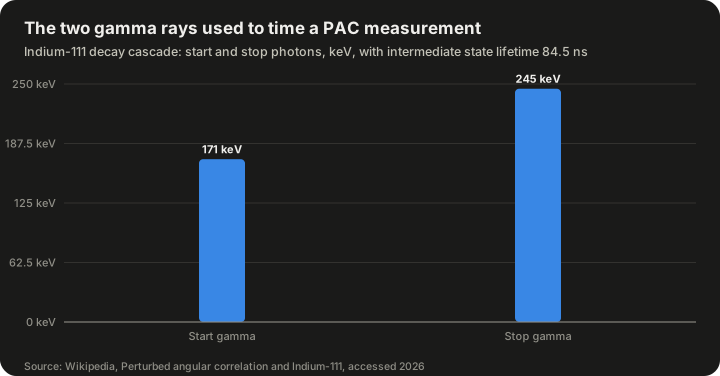
| Indium-111 PAC cascade | Value |
|---|---|
| Start gamma ray | 171 keV (171.3 keV in nuclear-medicine data, about 91% yield) |
| Stop gamma ray | 245 keV (245.4 keV, about 94% yield) |
| Intermediate state lifetime | 84.5 ns |
Source: Wikipedia articles on perturbed angular correlation and indium-111.
The measurement. Detectors, usually four in a plane at 90° to each other or six in an octahedral arrangement, record coincidences between start and stop photons. A count-rate ratio,
R(t) = 2[W(180°,t) − W(90°,t)] / [W(180°,t) + 2W(90°,t)],
is formed from coincidences at 180° and 90°, which cancels many experimental factors and leaves the hyperfine modulation.
What it yields. From the modulation, PAC extracts:
- the quadrupole coupling constant ν_Q = eQV_zz/h, which is independent of nuclear spin and therefore lets different isotopes of the same element be compared;
- the asymmetry parameter η;
- for magnetic sites, the Larmor frequency ω_L = g μ_N B/ħ, from which the magnetic field B follows.
A sharp single frequency set means all probes sit in one well-defined environment. Several frequency sets mean several distinct sites, such as a defect-free site and a site next to a defect. Damping of the modulation indicates a spread of environments or dynamic effects, such as a defect jumping around near the probe.
Strengths. PAC needs remarkably few probe atoms: about 10¹⁰ to 10¹² per measurement, with source activities of roughly 0.1–5 MBq. Unlike NMR and Mössbauer spectroscopy, it shows no signal attenuation at very high temperatures, so it can follow phase transitions and diffusion in hot samples. Probes can be introduced by ion implantation (the most common method), evaporation, diffusion, addition during synthesis, neutron activation or nuclear reaction.
Applications. PAC has been used to study semiconductors such as Si, InP, GaAs, InAs and ZnO, reviewed by Dogra, Byrne and Ridgway in 2009; oxides, including bixbyite-structure oxides and hafnium dioxide, reviewed by Pasquevich and Rentería in 2011; intermetallic compounds; surfaces and interfaces; phase transitions; magnetism; diffusion; nanomaterials; and frozen biological samples such as proteins.
Muon spin spectroscopy (μSR)
μSR is not a nuclear method, but it uses the same idea of a local spin probe. Positive muons, short-lived particles produced at accelerators, are implanted into a sample, where they come to rest at interstitial sites. Their spins precess in the local magnetic field, and when each muon decays it emits a positron preferentially along its spin direction, so the precession can be recorded. A key difference from NMR is that μSR uses an implanted spin rather than relying on the nuclei already present. Muon beams are available at facilities including PSI in Switzerland, TRIUMF in Canada, J-PARC in Japan and the ISIS Neutron and Muon Source / RIKEN-RAL in the United Kingdom.
Comparing the probes
Because each method relies on a particular nucleus or particle, the choice of technique often depends on which atoms are in the material.
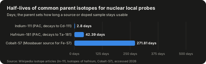
| Parent isotope | Half-life (days) | Decay | Used for |
|---|---|---|---|
| Indium-111 | 2.8048 | Electron capture to cadmium-111 | PAC probe |
| Hafnium-181 | 42.39 | Beta-minus decay to tantalum-181 | PAC probe |
| Cobalt-57 | 271.81 | Electron capture to iron-57 | Mössbauer source for iron studies |
Source: Wikipedia articles on indium-111, isotopes of hafnium and cobalt-57.
The half-life shapes how an experiment is run. An indium-111 sample loses half its activity in under three days, so it must be prepared and measured quickly. A hafnium-181 probe allows weeks of measurement. A cobalt-57 Mössbauer source, at roughly nine months' half-life, is a piece of laboratory equipment that can be used for many experiments before it must be replaced.
| Consideration | NMR | Mössbauer | PAC |
|---|---|---|---|
| Elements accessible | Many, if a suitable stable isotope exists | Limited to Mössbauer-active isotopes, mainly iron, tin, iodine, antimony | Limited to suitable cascade isotopes, mainly In/Cd and Hf/Ta |
| Sample amount | Usually relatively large | Moderate | Tiny numbers of probe atoms |
| High temperatures | Signal weakens | Recoil-free fraction falls | No attenuation at very high temperatures |
| Radioactivity | None | Source is radioactive; sample usually not | Sample contains the radioactive probe |
| Information | Chemical environment, EFG, local fields | Oxidation state, EFG, magnetic field | EFG, magnetic field, dynamics |
Worked examples
The following examples are hypothetical exercises using the formulas and constants above. The numbers are illustrative, not measurements of a real material, except where a published constant is used.
Example 1: How much activity does a PAC sample have?
Suppose a sample contains 10¹² atoms of indium-111, the upper end of the range quoted for PAC measurements.
- The decay constant is λ = ln 2 / t½.
- The half-life is 2.8048 days = 2.8048 × 86,400 s ≈ 242,335 s.
- So λ ≈ 0.6931 / 242,335 ≈ 2.86 × 10⁻⁶ per second.
- The activity is A = λN ≈ 2.86 × 10⁻⁶ × 10¹² ≈ 2.86 × 10⁶ decays per second, or about 2.9 MBq.
That falls inside the quoted working range of roughly 0.1–5 MBq, which shows how the probe-atom numbers and the activity figures fit together. After one half-life, 2.8 days, the activity would be about 1.4 MBq.
Example 2: From quadrupole coupling to PAC frequencies
For a probe state with spin I = 5/2, such as the intermediate state used in ¹¹¹Cd PAC, the quadrupole frequency is
ω_Q = eQV_zz / [4I(2I − 1)ħ].
With I = 5/2, the factor 4I(2I − 1) = 4 × 2.5 × 4 = 40. Since ν_Q = eQV_zz/h and ħ = h/2π, this gives ω_Q = 2πν_Q / 40.
Suppose, hypothetically, that a site has ν_Q = 100 MHz and an axially symmetric EFG (η = 0). Then:
- ω_Q = 2π × 100 MHz / 40 ≈ 15.7 million radians per second.
- For spin 5/2 with η = 0, the three observed frequencies are 6ω_Q, 12ω_Q and 18ω_Q, which satisfy the general rule ω₁ + ω₂ = ω₃.
- So ω₁ ≈ 94 Mrad/s, ω₂ ≈ 188 Mrad/s and ω₃ ≈ 283 Mrad/s, and indeed 94 + 188 ≈ 283 within rounding.
If a defect moved next to some of the probes and changed ν_Q at their sites, a second set of three frequencies would appear, and the relative amplitudes of the two sets would show what fraction of probes sit next to the defect.
Example 3: The energy scale of a Mössbauer spectrum
The Wikipedia article on Mössbauer spectroscopy gives the calculated separation of the two outermost lines of the six-line spectrum of iron foil as 10.6258 mm/s, and the conversion 1 mm/s = 48.075 neV for iron-57.
- The energy separation is 10.6258 × 48.075 neV ≈ 510.8 neV, or about 5.1 × 10⁻⁷ eV.
- That is consistent with the article's statement that magnetic hyperfine splittings are of order 10⁻⁷ eV.
- Compared with the 14.4 keV gamma-ray energy, the splitting is about 5.1 × 10⁻⁷ / 1.44 × 10⁴ ≈ 3.5 × 10⁻¹¹ of the photon energy.
This is why the method needs the extraordinary sharpness of recoil-free resonance: the effects being measured are a few parts in 10¹¹ of the gamma-ray energy.
Complementary non-nuclear methods
Nuclear probes are not the only way to study local structure. Two X-ray and neutron-based approaches are widely used, often alongside nuclear methods.
X-ray absorption fine structure (EXAFS)
When an X-ray photon is absorbed by an atom, it ejects a core electron. That electron's wave travels outward, scatters off neighbouring atoms and returns, interfering with itself and producing small oscillations in the absorption just above the absorption edge. These oscillations encode the distances to neighbouring atoms, their number (the coordination number) and their disorder. The modern form of the technique is associated with Sayers, Stern and Lytle, whose 1971 paper in Physical Review Letters introduced Fourier analysis of the signal.
EXAFS probes local structure within less than about 1 nm of the absorbing atom, and because each element has its own absorption edge, it is element-specific. It usually requires a tunable synchrotron X-ray source, with which an element can be detected at concentrations as low as a few parts per million; some laboratory instruments can now measure edges in the 5–30 keV range. The near-edge part of the spectrum, XANES, is sensitive to oxidation state and coordination environment.
Pair distribution function (PDF) analysis
The pair distribution function describes the probability of finding two atoms at a given separation. In total-scattering experiments, X-ray or neutron diffraction data are collected over a wide range and transformed to give the PDF. Unlike conventional crystallography, PDF analysis uses both the Bragg peaks and the diffuse scattering between them, and it is better suited to materials whose periodicity is broken by structural distortions, such as nanomaterials, amorphous solids and disordered thin films.
| Method | Element-specific? | Range probed | Main output |
|---|---|---|---|
| EXAFS | Yes | Within about 1 nm | Neighbour distances, coordination numbers, disorder |
| XANES | Yes | Immediate environment | Oxidation state, coordination geometry |
| Not inherently (total scattering) | Short to intermediate range | Distribution of interatomic distances | |
| NMR / Mössbauer / PAC | Yes (specific nucleus) | Dominated by nearest neighbours | Local fields, EFG, site symmetry |
In practice, researchers often combine methods. EXAFS might give the distance to the nearest neighbours of a dopant, PAC or Mössbauer spectroscopy might show whether the site is symmetric or distorted, and density functional theory calculations might test which proposed structure reproduces both.
Magnetic local structure
The same nuclear methods that measure EFGs can measure local magnetic fields, building up what the Wikipedia article calls a "magnetic local structure." In a magnetic material, the field at each nucleus depends on the magnetic moments of its own atom and its neighbours. A defect can change that field locally.
- In Mössbauer spectroscopy, the six-line magnetic pattern of iron-57 gives the field directly; metallic iron's 33 T internal field is a reference point.
- In PAC, the Larmor precession frequency gives the field at the probe.
- In NMR, the field shifts or splits the resonance.
- In μSR, the muon's precession gives the field at its interstitial site.
These measurements matter for technologies built on thin magnetic layers, such as the giant magnetoresistance read heads used in hard drives, where the properties of interfaces and defects between layers can determine how a device performs.
A short history of local-structure methods
The tools described above were developed over most of the twentieth century, largely independently, and only later came to be seen as a common toolkit for local structure.
| Year | Development |
|---|---|
| 1938 | Rabi observes nuclear magnetic resonance in molecular beams |
| 1940 | Hamilton publishes the theory of gamma-gamma angular correlation |
| 1946 | Bloch and Purcell extend NMR to liquids and solids |
| 1947 | Brady and Deutsch perform the first angular correlation experiment |
| 1949 | Knight reports the NMR shift in metals now named after him |
| 1953 | Abragam and Pound publish the theory of perturbed angular correlation in external fields |
| 1958 | Mössbauer discovers recoil-free gamma-ray resonance |
| Mid-1960s | Ion implantation makes it possible to insert probe atoms into almost any material |
| 1971 | Sayers, Stern and Lytle introduce Fourier analysis of EXAFS |
| 1979 | Kaufmann and Vianden review the EFG in non-cubic metals |
| 1980s onward | PAC becomes an established materials characterisation method |
| 2008 | First fully digital PAC spectrometer |
Sources: Wikipedia articles on NMR, PAC, Knight shift, Mössbauer spectroscopy and EXAFS; Kaufmann and Vianden (1979).
Two shifts in thinking stand out. The first was the move from using these effects to study nuclei to using nuclei to study materials. Early angular correlation experiments, for example, were designed to measure nuclear spins and parities; only later did physicists realise that the perturbations they had first treated as a nuisance were a rich source of information about the surrounding solid. The second was the growth of reliable calculation. For decades, interpreting a measured EFG required simplified models of the surrounding charges. Density functional theory now allows researchers to calculate the EFG for a proposed structure from first principles, turning a measured number into a strong test of a structural model.
Limitations
Local-structure methods are powerful but not universal.
| Limitation | Explanation |
|---|---|
| Limited choice of probes | Mössbauer and PAC work only with particular isotopes, so the probe may not be the element of greatest interest |
| The probe can perturb the site | A foreign probe atom, such as indium in a host where it is an impurity, may itself distort its surroundings |
| After-effects of decay | In PAC, electron capture decay of ¹¹¹In to ¹¹¹Cd can leave several electron holes at the probe, temporarily changing the local charge state |
| Indirect interpretation | Measured fields must be translated into structures, usually with the help of calculations |
| Radioactivity | PAC and Mössbauer require handling radioactive material and appropriate licensing |
| Facility access | EXAFS often needs a synchrotron; μSR needs a muon beam facility |
| Sensitivity of NMR | NMR signals are weak, and some nuclei are hard to observe |
None of these limits is fatal, but they explain why no single method dominates and why studies often combine several.
Common misconceptions
"If diffraction shows a perfect crystal, the material has no defects." Diffraction reports the average structure. A material can look perfect by diffraction and still contain the defects that control its properties.
"Local structure is just the unit cell." The unit cell is an average. Local structure is what a specific atom actually sees, which may differ from the average around a defect.
"Nuclear methods are about nuclear physics, not materials." The nuclear properties are only the instrument. The information obtained is about electrons and neighbouring atoms in the material.
"PAC and Mössbauer samples are dangerously radioactive." Activities are modest; the typical PAC range quoted is about 0.1–5 MBq. They still require proper radiation-safety procedures.
"The electric field matters for quadrupole interactions." It is the gradient of the field, not its strength, that couples to the quadrupole moment, and the gradient is zero for cubic symmetry.
Frequently asked questions
What does "local structure" mean in one sentence?
The arrangement of the nearest neighbours around a particular atom in a crystal or molecule.
Why can't X-ray diffraction see it?
Diffraction averages over vast numbers of atoms, so small fractions of atoms in unusual environments barely affect the Bragg peaks.
What is a hyperfine interaction?
The interaction between a nucleus and the electric and magnetic fields produced by its surroundings, which slightly shifts and splits the nuclear energy levels.
What is the electric field gradient?
The rate at which the electric field changes at the nucleus, described by the second derivatives of the electrostatic potential. It couples to nuclei with spin I ≥ 1 and is zero in a perfectly cubic environment.
Which technique should be used for iron compounds?
Iron-57 Mössbauer spectroscopy is the classic choice, because it reports oxidation state, site symmetry and magnetic field simultaneously.
Why is indium-111 popular for PAC?
Its decay to cadmium-111 produces a convenient two-gamma cascade (about 171 and 245 keV) with an 84.5 ns intermediate state, and its half-life of about 2.8 days is long enough for experiments but short enough for manageable handling. Indium-111 is also widely used in nuclear medicine for imaging.
Is local structure only about defects?
No. Defects are the most common reason to study it, but local structure also matters in perfect crystals with more than one kind of site, as in magnetite, whose two iron sites give two distinct Mössbauer patterns, and in glasses, liquids and nanoparticles that have no long-range order at all.
Can local structure be calculated?
Yes. Density functional theory is now an important tool for calculating EFGs and local fields for candidate structures, which are then compared with measurements.
Sources
- Local structure – Wikipedia
- Electric field gradient – Wikipedia
- Hyperfine structure – Wikipedia
- Perturbed angular correlation – Wikipedia
- Mössbauer spectroscopy – Wikipedia
- Rudolf Mössbauer – Wikipedia
- Nuclear magnetic resonance – Wikipedia
- Knight shift – Wikipedia
- Nuclear quadrupole resonance – Wikipedia
- Muon spin spectroscopy – Wikipedia
- Extended X-ray absorption fine structure – Wikipedia
- Pair distribution function – Wikipedia
- Indium-111 – Wikipedia
- Isotopes of hafnium – Wikipedia
- Cobalt-57 (Isotopes of cobalt) – Wikipedia
- Kaufmann and Vianden (1979), The electric field gradient in noncubic metals, Reviews of Modern Physics 51, 161
- Pasquevich and Rentería (2011), PAC study of EFGs at impurity sites in oxides, Defect and Diffusion Forum 311, 62
- Dogra, Byrne and Ridgway (2009), PAC for characterising semiconductors, Journal of Electronic Materials
- AG Hofsäss, PAC probes 111In and 181Hf – University of Göttingen