Insulation is sold on numbers. A roll of mineral wool, a board of foam or a jacket for a steam pipe comes with a thermal conductivity or an R-value measured in a laboratory under controlled conditions. But once insulation is installed, the question changes. Is it performing as specified? Has it been compressed, soaked, damaged or badly fitted? Is a wall losing the heat the design calculations predicted, or more, or less?
Answering those questions in the field means measuring heat flow directly, on the real installation, while it is in service. The standard tool for this is the heat flux sensor, also called a heat flux transducer (HFT) or heat flux plate (HFP): a thin, flat device that produces a small voltage proportional to the heat passing through it. Taped or pressed against a surface, together with temperature sensors on either side, it allows the heat flux, the thermal resistance and the thermal transmittance (U-value) of the insulated element to be calculated.
The Wikipedia article on this topic focuses on on-site (in-situ) measurement of flat surfaces using the now-withdrawn ASTM C1041 practice for industrial insulation. This article covers that method and places it in its wider context: the physics of heat flow through insulation, how heat flux sensors work, the laboratory methods that establish insulation's rated performance, the building-envelope standards (ISO 9869-1, ASTM C1046 and C1155) that are now the most common application, the error sources that research has quantified, and what field studies have learned about how long a measurement must run.
Basic concepts
Heat flux
Heat flux, written q, is the rate of heat flow per unit area, measured in watts per square metre (W/m²). It is the quantity a heat flux sensor measures. If a wall loses 20 W through each square metre of its surface, the heat flux through it is 20 W/m².
Thermal conductivity
Thermal conductivity, written λ (lambda) or k, is a material property: the heat flux that flows through a 1 m thickness of the material when the temperature difference across it is 1 K. Its unit is W/(m·K). Good insulators have low conductivity. The table below gives representative room-temperature values from the Wikipedia list of thermal conductivities.
| Material | Thermal conductivity, W/(m·K), near room temperature |
|---|---|
| Air (still) | 0.024–0.026 |
| Silica aerogel | about 0.02 (other sources lower) |
| Polyurethane foam | 0.03 |
| Expanded perlite | 0.031 |
| Expanded polystyrene (EPS) | 0.03–0.046 |
| Mineral wool | about 0.04 (rock wool 0.034–0.042) |
| Cork | 0.04–0.07 |
| Pine wood | about 0.10 |
| Brick | 0.15–1.31 |
| Concrete | 0.8–2.5 |
Source: Wikipedia, "List of thermal conductivities." Values vary with density, moisture and temperature.
Most insulating materials work by trapping air or another gas in small cells or between fibres, so their conductivity is close to that of still air. The ranges are wide because conductivity depends on density, moisture content and temperature, which is one reason why measuring installed performance matters.
Thermal resistance and U-value
For a layer of thickness D, the thermal resistance is R = D / λ, in m²·K/W. Higher is better. Resistances of layers in series add up.
The thermal transmittance, or U-value, is the heat flux per kelvin of temperature difference between the air on one side and the air on the other, in W/(m²·K). It includes the surface resistances (the thin layers of still air at each face) as well as the resistance of the material. Lower is better. For a simple element, U = 1 / Rtotal.
The distinction matters in measurement:
- Using surface temperatures on each face gives the thermal resistance of the element itself.
- Using air temperatures on each side gives the U-value, which includes the surface resistances.
Steady state and why it is hard to achieve
All these definitions assume steady state: temperatures that do not change with time, so the heat flowing in on one side equals the heat flowing out on the other. In a laboratory, steady state can be created deliberately. In the field, it almost never exists. Outdoor temperatures swing day and night, the sun heats walls, wind changes surface heat transfer, and processes cycle. A massive wall stores and releases heat, so the heat flux at its inner surface at any moment reflects conditions hours or days earlier.
The central problem of in-situ heat flux measurement is how to extract a steady-state property from data collected under non-steady conditions. The answer is usually some form of averaging over a long enough period, or a dynamic model that accounts for heat storage.
How a heat flux sensor works
The thermopile principle
Most heat flux sensors are built around a thermopile: many thermocouples connected in series, with alternate junctions on the top and bottom faces of a thin plate. When heat flows through the plate, a small temperature difference develops across it, and each thermocouple produces a tiny voltage proportional to that difference. Connecting many in series adds the voltages together.
The Wikipedia article on heat flux sensors notes that thermopiles are stable, have low electrical resistance and give zero output for zero input, but have low sensitivity. The sensor needs no power supply.
The heat flux is calculated from the output voltage V and the sensor's calibrated sensitivity S:
q = V / S
This is the same relation given in the Wikipedia article on heat flux measurements of insulation, with S in V/(W/m²).
A real example: the Hukseflux HFP01
A widely used sensor for building and insulation work is the Hukseflux HFP01, which was used in the UK government-funded study discussed below. The manufacturer's specifications are:
| Parameter | Value |
|---|---|
| Nominal sensitivity | 60 × 10⁻⁶ V/(W/m²), i.e. 60 µV per W/m² |
| Measurement range | −2,000 to +2,000 W/m² |
| Sensor thermal resistance | 71 × 10⁻⁴ m²·K/W |
| Thickness | 5.4 mm |
| Sensing area | 8 × 10⁻⁴ m² |
| Guard width to thickness ratio | 5 |
| Calibration uncertainty | ±3% (k = 2) |
| Operating temperature | −30 to +70 °C |
Source: Hukseflux HFP01 product specifications. The manufacturer states the guard width meets ISO 9869 requirements and that the sensor can be used for measurements under ISO 9869, ASTM C1046 and ASTM C1155.
The Wikipedia heat flux sensor article gives the HFP01's diameter as 80 mm.
Worked example: from voltage to heat flux (hypothetical)
Suppose an HFP01 with exactly the nominal sensitivity reads 1.2 mV on the inside face of a wall.
q = 1.2 × 10⁻³ V / 60 × 10⁻⁶ V/(W/m²) = 20 W/m²
On an insulated steam pipe or vessel, fluxes are higher. If the same sensor read 6.0 mV, the flux would be 6.0 × 10⁻³ / 60 × 10⁻⁶ = 100 W/m².
The voltages are small, which is why heat flux sensors are read with sensitive dataloggers or integrating voltmeters. The Wikipedia heat flux sensor article mentions voltmeter resolution of ±2 µV or better for calibration work.
Other sensor types
The Wikipedia heat flux sensor article lists several other designs, mostly for higher heat fluxes or faster events than insulation testing involves:
- Gardon gauges (circular-foil gauges), common in fire and furnace testing.
- Schmidt-Boelter gauges, with a wire-wound geometry.
- Thin-film thermopiles and atomic layer thermopiles, with response times in microseconds and ranges up to 100 MW/m².
- Self-calibrating sensors with an integrated heater.
For insulation and building work, flat thermopile plates like the HFP01 dominate.
Response time
A heat flux sensor has thermal mass, so it takes time to respond to a change. The Wikipedia article gives its time constant as τ = d²ρcp / λ, where d is thickness, ρ density, cp specific heat and λ conductivity. Because response time scales with the square of thickness, thicker sensors are much slower. The same article notes it generally takes several minutes to reach 95% of the final response. That is fast compared with the hours-to-days timescales of building heat flow, but it matters for transient industrial measurements.
Laboratory measurement: where rated values come from
Before discussing field measurement, it helps to know how insulation is tested in the laboratory, because field measurements are always compared with these values.
The guarded hot plate (ASTM C177)
The guarded hot plate is the reference method. A flat specimen is placed between a heated plate and a cooled plate, and the electrical power supplied to the heater is measured directly. A surrounding "guard" heater kept at the same temperature prevents heat leaking sideways, so all the measured power flows through the specimen. Because the heat flow is determined from electrical power rather than from a calibrated sensor, ASTM describes the method as primary, or absolute. The ASTM C177 standard states that comparative methods cannot be more accurate than it, and recommends it as the procedure in cases of dispute.
The heat flow meter apparatus (ASTM C518)
The heat flow meter apparatus places a specimen between two plates at different temperatures and measures the heat flux with heat flux transducers. It is faster than the guarded hot plate and widely used for production testing, but it is comparative: the transducers must be calibrated against reference materials of known conductivity, themselves measured on a guarded hot plate. Testing laboratories note that results from this method are used to demonstrate compliance with the US Federal Trade Commission's R-value Rule for insulation products.
Why laboratory values differ from field performance
Laboratory specimens are clean, dry, flat and tested at a controlled mean temperature. Installed insulation may be compressed, have gaps at joints, contain moisture, sit at very different temperatures, or have fasteners and supports running through it. These are exactly the effects in-situ measurement is designed to reveal.
In-situ measurement of industrial insulation: ASTM C1041
Scope
ASTM C1041, "Standard Practice for In-Situ Measurements of Heat Flux in Industrial Thermal Insulation Using Heat Flux Transducers," is the practice on which the Wikipedia article is based. According to the reference listed there, it was withdrawn in 2019. The Wikipedia article confines itself to flat surfaces; pipes, which need different geometry, are excluded.
The aim is to measure heat flux q, or apparent thermal conductivity λ, under pseudo-steady-state conditions with minimal disturbance to the system.
Choosing the measurement location
The Wikipedia summary of the practice sets out several requirements:
- Place the sensor on a section of insulation that is representative of the whole system, not near a boiler inlet or outlet or a heating element, where local conditions are unusual.
- Shield the sensor from irrelevant heat sources such as direct sunlight.
- Attach the sensor with thermal paste or another conductive material so there is no air gap.
- Match the sensor's surface emittance to that of the surface as closely as possible, so it exchanges radiant heat in the same way.
Preliminary measurements
Before logging begins:
- Measure the insulation thickness to the nearest millimetre.
- Record ambient conditions if relevant: humidity, air movement and precipitation.
- Measure the surface temperature next to the sensor and the process-side temperature (the hot face of the insulation).
Collecting and processing data
The sensor is connected to a datalogger or integrating voltmeter. The operator waits until conditions reach pseudo-steady state, then averages readings over a short period. Measurements should be repeated at several relevant locations.
Two calculations follow. The heat flux is q = V / S. The apparent thermal conductivity is
λ = q D / (t₁ − t₂)
where D is the insulation thickness, t₁ the process-side (hot) surface temperature and t₂ the outer surface temperature measured near the sensor. If D is recorded in millimetres, it must be converted to metres to give λ in W/(m·K).
Worked example (hypothetical)
An insulated flat duct wall carries hot process air. The insulation is 50 mm thick. The hot face is at 150 °C and the outer surface, next to the sensor, is at 30 °C. The sensor reads 6.0 mV with a sensitivity of 60 µV/(W/m²).
- Heat flux: q = 6.0 × 10⁻³ / 60 × 10⁻⁶ = 100 W/m²
- Temperature difference: 150 − 30 = 120 K
- Apparent conductivity: λ = 100 × 0.050 / 120 = 5.0 / 120 ≈ 0.042 W/(m·K)
That is in the range expected for mineral wool, which suggests the insulation is performing broadly as expected at this location. If the result had been, say, 0.08 W/(m·K), it would point to wet, compressed or damaged insulation, or to a measurement problem worth investigating. The value is "apparent" because it is an average over a range of temperatures and may include effects such as convection within the insulation.
Error sources named in the practice
The Wikipedia summary lists the main ways the measurement can go wrong:
- Emittance mismatch between sensor and surface, which changes how the sensor exchanges radiant heat.
- Air or other material between the sensor and the surface, which adds a thermal resistance.
- Unshielded external heat sources, such as solar radiation.
- Poor placement near inlets, outlets or heating elements.
The article notes that overall precision depends on the choice of sensor and test section and on external conditions, and gives no single numeric tolerance.
Early literature
The references cited in the Wikipedia article show how long this technique has been in use:
- C. F. Gilbo, "Conductimeters, Their Construction and Use," ASTM Bulletin No. 212 (February 1956).
- H. F. Poppendiek, "Why Not Measure Heat Flux Directly?" Environmental Quarterly 15, No. 1 (1969).
- G. Johannesson, "Heat Flow Measurements, Thermoelectrical Meters, Function Principles, and Sources of Error," Lund Institute of Technology, Report TUBH-3003 (1979), translated in draft for the US Army Corps of Engineers in 1982.
In-situ measurement of building envelopes
The largest application of heat flux measurement today is in buildings, where the question is whether walls, roofs and floors lose heat as calculated. Two families of standards apply.
ASTM C1046 and C1155
ASTM C1046 covers the use of heat flux transducers and temperature transducers to measure the in-situ dynamic or steady-state thermal behaviour of opaque building envelope components. It recommends using infrared thermography to locate appropriate sites for the sensors, unless subsurface conditions are already known, and gives guidance on placing sensors so that the results represent more than just the instrumented spot.
ASTM C1155 covers how to compute thermal resistance from the C1046 data. It presents two techniques, the summation technique and the sum of least squares technique, and allows other properly validated methods. It notes that each result applies only to the instrumented subsection, and that combining subsections to characterise a whole building is outside its scope. It also cautions that field measurements may not achieve the accuracy of laboratory apparatus.
ISO 9869-1
Internationally, the reference is ISO 9869, "Thermal insulation: Building elements: In-situ measurement of thermal resistance and thermal transmittance." Part 1 (2014) covers the heat flow meter method. It describes an average method and a dynamic method.
The average method divides the sum of the measured heat fluxes by the sum of the measured temperature differences over the test period:
U ≈ Σq / Σ(Ti − Te)
As summarised by Juricic and colleagues (2020), the standard sets three conditions that must all be met before a test can end:
- The test must last 72 hours or longer.
- The U-value at the end of the test must not deviate by more than 5% from the value obtained 24 hours earlier.
- The U-value obtained from the first two-thirds of the data and from the last two-thirds must not deviate by more than 5%.
A further condition, described in documentation of the standard, is that the average method applies only when the heat stored in the element is the same at the start and end of the test, and that the sensor must not be exposed to direct sunlight. For heavy elements, the analysis period should be an integer multiple of 24 hours.
The dynamic method fits a model that accounts for heat storage, which can give reliable results from shorter or more variable datasets.
Worked example: the average method (hypothetical)
A wall is monitored for three days with the following daily averages:
| Day | Mean heat flux (W/m²) | Indoor air (°C) | Outdoor air (°C) | Difference (K) |
|---|---|---|---|---|
| 1 | 24 | 20 | 6 | 14 |
| 2 | 30 | 20 | 3 | 17 |
| 3 | 21 | 20 | 8 | 12 |
- Sum of heat flux: 24 + 30 + 21 = 75
- Sum of temperature differences: 14 + 17 + 12 = 43
- U-value estimate: 75 / 43 ≈ 1.74 W/(m²·K)
The daily ratios are 24/14 ≈ 1.71, 30/17 ≈ 1.76 and 21/12 = 1.75, so the estimate is fairly stable. In practice, data are logged every few minutes and the convergence checks above are applied to the running estimate.
What research has measured about accuracy
The BRE study for the UK government
The Building Research Establishment (BRE) carried out a research programme for the UK Department of Energy and Climate Change (DECC) on heat losses from solid-walled homes, building on field trials including one BRE ran in 2011. Field trials had suggested that solid walls lose less heat than generally assumed. A related BRE report notes that in-situ U-values of solid walls were measured lower than the generally assumed value of 2.1 W/(m²·K), and BRE carried out in-situ wall measurements in approximately 300 dwellings. Before relying on those results, BRE needed to know whether the measurement method itself was biased.
The 2016 report "In situ U-value measurement method review," led by Tim Ward and Sean Doran, ran seven tests: comparisons against hot-box measurements at the National Physical Laboratory (NPL), the effect of surface roughness, reproducibility of the sensor's contact layer, fixing methods, the effect of sunlight, and the vertical and horizontal stratification of indoor air temperature.
Hot-box comparison. In NPL's rotatable hot box, the heat flux measured by HFP01 plates was on average 3.8% lower than the hot-box value on a smooth plasterboard surface and 5.7% lower on an embossed wallpaper surface. Thermal modelling indicated a systematic error of −8.0% from the presence of the plate itself. BRE concluded that measured U-values using HFP01 plates should be corrected by multiplying by 1.05, a +5% correction. BRE also noted that the variation in systematic error between individual plates, from about +1% to about −7%, was within the 5% inaccuracy of the manufacturer's calibration system.
Steady state versus dynamic conditions. BRE built a solid brick wall in the hot box and measured it under both steady and cycling temperatures, uninsulated and with external insulation installed well and badly. The results show that the measured U-value represents the underlying steady-state property even under varying conditions.
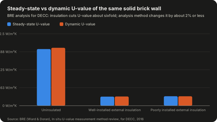
| Wall 3 condition | Steady-state U-value (W/m²K) | Dynamic U-value (W/m²K) | Change |
|---|---|---|---|
| Uninsulated | 1.970 | 2.014 | +2.2% |
| Well-installed external insulation | 0.315 | 0.320 | +1.6% |
| Poorly installed external insulation | 0.329 | 0.328 | −0.0% |
Source: BRE (Ward and Doran), "In situ U-value measurement method review," for DECC, 2016, Table 7.
The chart makes two points at once. Insulating the wall cut its U-value about sixfold (1.970 to 0.315). And the difference between steady and dynamic measurement was 2.2% or less, far smaller than the effect being measured. The difference between well- and poorly-installed insulation (0.315 versus 0.329, about 4%) is small in this test, but in the same range as the measurement corrections, which shows how hard it is to detect modest installation defects from heat flux alone.
Fixing the sensor. BRE found that a thin layer of petroleum jelly and cling film gave good thermal contact on both smooth and embossed surfaces, and that removing and reapplying it gave consistent results even with different operators. Double-sided tape was unreliable on dusty surfaces. Duct tape over the plate gave better contact but itself affected the U-value, possibly through air pockets or reduced emissivity.
Sunlight and temperature difference. U-values were fairly stable when the inside-outside temperature difference exceeded 10 K. Measurements with smaller differences might be possible if the sun was not shining on the wall, but BRE described this as only indicative. On an unshaded south facade, BRE advised measuring for longer than the recommended two weeks to collect enough suitable days.
Sensor height. Vertical position did not materially affect the result, provided the plate was at least 200 mm from the ceiling and floor and the indoor temperature was measured next to the plate.
Air temperature position. In colder months, air temperature measured 10 mm from the wall could be about 2% lower than further away, leading to about a 2% overestimate of U-value. BRE recommended measuring indoor air temperature at least 20 mm from the wall surface.
How long a test must run
The ISO minimum of 72 hours is widely regarded as too short for many walls. Several studies have quantified this.
- Gaspar and colleagues, as summarised by Juricic and colleagues, found that the ISO conditions secure convergence within 4 to 5 days for both the average and dynamic methods on the walls they studied.
- Gori and colleagues, also as summarised by Juricic, found that applying the ISO criteria, up to 10 days were needed to reach stabilisation in autumn and winter, and longer in warmer seasons. With a resistance-capacitance (RC) model, shorter datasets sometimes sufficed, implying the ISO conditions might be too conservative when applied to other analysis methods.
- Rodler and colleagues, also summarised by Juricic, found that the temperature difference mattered more than the length of the dataset.
- BRE worked with a recommended field period of two weeks.
- Du and Pilkington (2026) monitored a recently insulated cavity brick wall in Liverpool with a design U-value of 0.18 W/(m²·K) for 130 days, logging every 10 minutes, and applied the average method to 13,687 candidate time windows. Only 5–10% of 72-hour windows met the convergence criteria, and among those the mean absolute error against long-duration references was about 32%. They found 14 days necessary for indicative results and 28 days for accuracy within ±5%.
At whole-building scale, Juricic and colleagues used simulation of a one-storey house to conclude that 11 days of data were needed for a robust estimate of overall thermal resistance under variable weather. Because that figure applies to the whole building envelope rather than a single wall, it is not directly comparable.
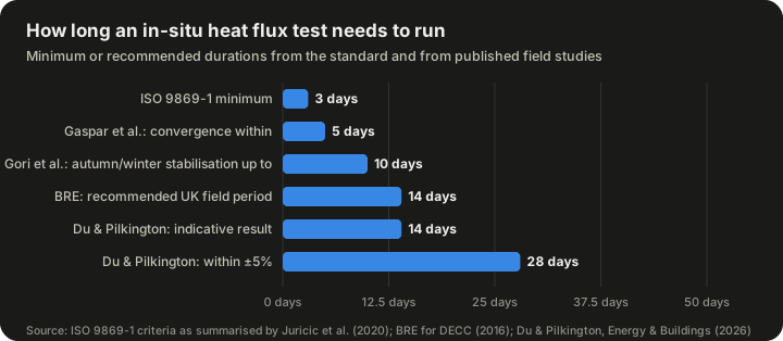
| Source | Duration | What it refers to |
|---|---|---|
| ISO 9869-1 | 3 days (72 h) | Minimum test length, with stability criteria |
| Gaspar et al. | within 4–5 days | Convergence with ISO criteria |
| Gori et al. | up to 10 days | Stabilisation in autumn and winter |
| BRE (2016) | 14 days | Recommended field period |
| Du & Pilkington (2026) | 14 days | Indicative result on a low U-value wall |
| Du & Pilkington (2026) | 28 days | Accuracy within ±5% |
Sources: ISO 9869-1 as summarised by Juricic et al. (2020); BRE for DECC (2016); Du and Pilkington, Energy & Buildings 369 (2026).
The evidence on what drives duration is not entirely one-directional. In one study by Gaspar and colleagues, walls with higher actual transmittance converged more slowly; Du and Pilkington, by contrast, cite another Gaspar study showing that facades with U-values below 0.5 W/(m²·K) need substantially longer tests, and they report that heavyweight and highly insulated walls may require 7 to 21 days. What the studies agree on is that 72 hours is often not enough. Du and Pilkington note that the 72-hour threshold was established when uninsulated walls lost heat far more rapidly than today's retrofits, and they propose a minimum duration that depends on wall type.
Moisture
Du and Pilkington also found that moisture was decisive. Wet periods inflated measured U-values by 13–16%, with recovery of 4–6 mW/(m²·K) per consecutive dry day. They recommend mandatory dry-spell preconditioning before testing. Moisture increases the conductivity of many materials, and evaporation and condensation within a wall carry latent heat that a heat flux sensor records as additional flow.
The performance gap
Measured and designed performance frequently disagree. Du and Pilkington cite a meta-analysis by O'Hegarty and colleagues of envelopes with design U-values below 0.3 W/(m²·K), in which 93% of tests showed underperformance; in their own campaign of ten measurements on highly insulated envelopes, nine of ten underperformed, with an average deviation exceeding 100%. Du and Pilkington caution that percentage deviations are amplified when the design U-value is small. In their own Liverpool wall, the measured values of 0.206 and 0.188 W/(m²·K) exceeded the 0.18 design value by only 0.026 and 0.008 W/(m²·K) in absolute terms, which is why they propose combining absolute and relative tolerances when judging whether a wall meets its design.
The BRE work illustrates the opposite direction for old solid walls, which have often measured better than assumed. Either way, the gap between calculation and measurement is the reason in-situ heat flux testing exists.
The disturbance a sensor causes
A heat flux sensor is not invisible. It adds a small thermal resistance to the surface, changes local radiation exchange and may alter air movement. This diverts some heat around the sensor, so it measures slightly less flux than would flow without it. The BRE modelling quantified this effect as a systematic error of about −7% to −8% for the configurations studied.
A simple illustration (hypothetical): the HFP01's thermal resistance is 0.0071 m²·K/W. For a wall whose surface-to-surface resistance is 0.5 m²·K/W, the sensor adds about 0.0071 / 0.5 ≈ 1.4% to the local resistance. For a well-insulated wall with a resistance of 5 m²·K/W, the added resistance is only about 0.14%. But the total disturbance also depends on edge effects, contact quality and emissivity, which is why BRE's modelled and measured errors were larger than this simple ratio suggests. The guard area around the sensing element, specified as a ratio of guard width to thickness, exists to reduce edge effects.
Planning a measurement campaign
Combining the standards and research findings gives a practical checklist.
Before installing sensors
- Define the question. Is the aim to check a specification, compare before and after a retrofit, find a defect, or calibrate an energy model?
- Find representative locations. ASTM C1046 recommends infrared thermography to locate sensor sites. Avoid thermal bridges (studs, lintels, fixings) unless they are the subject of the test.
- Check the season. For buildings, measurement is most reliable when the temperature difference is large. BRE found results stable above 10 K.
- Check moisture history. Following Du and Pilkington, a period of dry weather before testing reduces moisture bias.
Installing sensors
- Fix the heat flux sensor to the surface with good thermal contact. BRE found petroleum jelly and cling film effective in homes; the industrial practice calls for thermal paste or another conductive material.
- Avoid placing sensors within 200 mm of ceilings or floors.
- Measure indoor air temperature next to the sensor, at least 20 mm from the wall surface.
- Shield sensors from direct sun, or choose a shaded facade.
- Match emittance where possible.
- Record insulation thickness and sensor positions.
Running the test
- Log heat flux and temperatures at short intervals for the full period.
- Plan for at least two weeks for typical walls, and longer for highly insulated or sunlit walls, following the evidence above.
- Note weather, occupancy and heating patterns.
Analysing the data
- Apply the ISO 9869-1 average method and check its convergence criteria, or use a dynamic method.
- Apply any sensor correction established for the equipment (BRE recommended 1.05 for HFP01 plates in its configuration).
- Report the uncertainty, not just a single number.
Industrial applications
Heat flux measurement is used well beyond building walls. The Wikipedia heat flux sensor article lists industrial uses including aluminium smelting, boilers, blast furnaces and flare systems, as well as aerospace and combustion research.
For industrial insulation, the questions are typically:
- Is the insulation still effective? Over years of service, insulation can be soaked by leaks, crushed, or degraded by heat. Comparing apparent conductivity with the original specification reveals deterioration.
- How much energy is being lost? Multiplying heat flux by surface area gives heat loss in watts, which can be translated into fuel cost and used to justify reinsulation.
- Is the surface safe? Surface temperature and heat flux together indicate whether a surface poses a burn risk.
Worked example: estimating heat loss (hypothetical)
A flat-sided tank has 40 m² of insulated surface. Heat flux measured at several representative points averages 100 W/m².
- Heat loss: 100 W/m² × 40 m² = 4,000 W, or 4 kW.
- Over a year of continuous operation (8,760 hours): 4 kW × 8,760 h = 35,040 kWh.
If reinsulation halved the flux, the saving would be about 17,520 kWh per year. Such estimates are only as good as the representativeness of the measurement points, which is why the industrial practice stresses measuring at several relevant locations.
Limitations of the technique
It measures a point, not a building. A heat flux sensor covers a small area, about 8 cm² of sensing area for the HFP01. ASTM C1155 explicitly states that each result applies only to the instrumented subsection. Extending results to a whole wall requires knowledge of its uniformity, ideally from thermography.
It needs a temperature difference. With little temperature difference, the heat flux is small and the signal-to-noise ratio poor. This limits building measurements to the heating season in most climates and makes low U-value walls harder to measure.
It needs time. Days to weeks for buildings, as discussed above.
It is sensitive to installation. Poor contact, sunlight, wrong emittance, or a sensor placed on a thermal bridge can all distort results.
Heat storage complicates interpretation. Heavy walls store and release heat, so instantaneous readings are meaningless. Long averages or dynamic models are needed.
Moisture adds uncertainty. Moisture in the wall changes both its conductivity and the latent heat flow, with Du and Pilkington measuring 13–16% inflation during wet periods.
Sensor calibration is a floor on accuracy. HFP01 calibration uncertainty is ±3% (k = 2) according to the manufacturer, and BRE referred to a 5% inaccuracy in the calibration system. Field results cannot be more accurate than this.
Common misconceptions
"A heat flux sensor measures temperature." It measures heat flow, using a temperature difference across itself. The surface temperature must be measured separately.
"Three days is always enough." The ISO minimum is a minimum, and research shows many walls need two to four weeks.
"A measured U-value is the true U-value." It is an estimate with uncertainty from calibration, installation, sensor disturbance, weather, storage and moisture. BRE found a systematic bias of about −4% to −8% in its configuration.
"The laboratory value is what you get installed." Laboratory values are for clean, dry, flat specimens. Installed performance can be worse or, for old masonry, sometimes better than assumed.
"Heat flux sensors work anywhere on the wall." Placement near corners, ceilings, floors, studs or fixings, or in sunlight, changes the result.
"More insulation is easier to measure." Generally it is harder, because the heat flux is smaller; Du and Pilkington found a low U-value wall needed 14 to 28 days.
Frequently asked questions
What is the difference between heat flux and heat flow?
Heat flow is the total rate of heat transfer, in watts. Heat flux is heat flow per unit area, in W/m². A sensor measures flux; multiplying by area gives flow.
What is the difference between R-value and U-value?
R-value is thermal resistance (higher is better) and U-value is thermal transmittance (lower is better). For a simple element, U = 1 / R, where R includes the surface air resistances.
Can heat flux measurement be done in summer?
It is difficult. BRE found results stable when the temperature difference exceeded 10 K and only indicative below that, and only when the sun was not on the wall.
Is ASTM C1041 still current?
According to the reference cited in the Wikipedia article, it was withdrawn in 2019. ASTM C1046 and C1155, and ISO 9869-1, remain the main in-situ standards for building envelopes.
How do I attach a heat flux sensor to a wall without damaging it?
BRE found a thin layer of petroleum jelly on cling film gave good contact on smooth and embossed surfaces, with consistent results when reapplied. Tape over the sensor itself affected the reading.
Why do my readings swing wildly from hour to hour?
Because buildings are not in steady state. Outdoor temperature, sun, wind and heating cycles change the flux constantly, and heavy walls store heat. The ISO average method and dynamic methods are designed to extract a steady-state value from this variation.
Can a heat flux sensor be used on pipes?
Yes, but pipes need different geometry and corrections. The Wikipedia article and the ASTM C1041 summary cover flat surfaces only.
How accurate are in-situ U-value measurements?
It depends on duration, conditions and installation. Du and Pilkington found mean absolute errors of about 32% for 72-hour windows on a low U-value wall, improving to within ±5% at 28 days. BRE found systematic bias of a few percent that can be corrected.
Summary
Heat flux measurement turns insulation from a specification into something that can be checked in place. A thin thermopile sensor, read with a sensitive logger and combined with temperature measurements, yields the heat flux, the apparent thermal conductivity, the thermal resistance or the U-value of an installed element. In industry, the now-withdrawn ASTM C1041 practice set out how to do this on flat insulated surfaces; in buildings, ASTM C1046 and C1155 and ISO 9869-1 are the main references. Research has put numbers on the method's limits: a few percent of systematic bias from the sensor itself, stable results only when temperature differences exceed about 10 K, test durations of two to four weeks rather than three days for modern well-insulated walls, and moisture effects of more than 10%. Used with those limits in mind, the technique remains the most direct way to find out how much heat an insulated surface is really losing.
Sources
- Heat flux measurements of thermal insulation (Wikipedia)
- Heat flux sensor (Wikipedia)
- List of thermal conductivities (Wikipedia)
- BRE (Ward, T. and Doran, S.), Solid wall heat losses and the potential for energy saving: In situ U-value measurement method review, for DECC, 2016 (GOV.UK)
- BRE, Solid wall heat losses: Nature of solid walls in situ (GOV.UK)
- Du, H. and Pilkington, A. (2026). Adapting ISO 9869-1 for post-retrofit low U-value walls: Evidence from 130 days of continuous in-situ monitoring. Energy & Buildings 369 (LJMU Research Online)
- Juricic, S. et al. (2020). Influence of weather natural variability on the thermal characterisation of a building envelope (arXiv:2011.13593)
- Hukseflux HFP01 heat flux sensor specifications
- ASTM C1155-95(2021) Standard Practice for Determining Thermal Resistance of Building Envelope Components from the In-Situ Data (ANSI Webstore)
- GSO ASTM C1046 Standard Practice for In-Situ Measurement of Heat Flux and Temperature on Building Envelope Components
- ASTM C177-19 Standard Test Method for Steady-State Heat Flux Measurements by Means of the Guarded-Hot-Plate Apparatus (ASTM)
- ASTM C518 Steady-State Thermal Transmission Properties by Heat Flow Meter Apparatus (Intertek)