Current sensing is the family of techniques used to measure electric current. It sounds like a narrow subject, but almost every piece of modern electrical equipment depends on it. A phone charger measures current to decide when a battery is full. A motor drive measures current many thousands of times per second to control torque. A utility meter measures current to bill a household. A particle accelerator measures the current in its magnets so precisely that errors are counted in parts per million. Protection relays measure current to decide, within a fraction of a second, whether a fault has happened and a breaker must open.
The range of currents involved is enormous. The Wikipedia article on the subject notes that current sensing covers everything from picoamperes to tens of thousands of amperes. No single sensor can cover that span, so engineers choose between several physical principles, each with its own strengths, weaknesses and costs. The main choices are:
- Resistive shunts, which use Ohm's law: pass the current through a small, known resistance and measure the voltage across it.
- Current transformers and Rogowski coils, which use Faraday's law of induction: a changing current produces a changing magnetic field, which induces a voltage in a nearby coil.
- Magnetic field sensors, such as Hall-effect devices, fluxgates and magnetoresistive sensors, which measure the magnetic field that any current produces and infer the current from it.
- Optical sensors, which use the Faraday effect: a magnetic field rotates the polarisation of light travelling through glass or optical fibre.
This article explains how each method works, what limits its accuracy and bandwidth, where it is used, and how engineers choose between them. It also covers the precision end of the field, where the accelerator community developed instruments that remain the reference for high-accuracy direct-current measurement.
Why current sensing matters
Current is one of the two quantities, along with voltage, that define electrical power. Measuring voltage is usually straightforward: you connect a high-impedance voltmeter across two points and it draws almost nothing. Measuring current is harder because current flows through a conductor. To measure it you must either put something in its path, which disturbs the circuit, or detect it indirectly through its magnetic field.
Current measurements serve four broad purposes.
Control. Power electronic converters, motor drives and battery chargers regulate current directly. In a motor, torque is proportional to current, so a drive that controls current controls torque. In a battery charger, the charging current must be held within the battery's safe limits.
Protection. Fuses and circuit breakers exist because excessive current causes overheating and fire. Electronic protection goes further: a power supply can shut down within microseconds if it detects an overcurrent, and a grid protection relay compares current readings across a transmission line to detect faults.
Metering and billing. Utility meters measure current and voltage to calculate energy. Accuracy here has direct financial consequences, which is why metering instruments are covered by formal accuracy classes.
Monitoring and diagnosis. Measuring current lets engineers see how equipment is behaving, detect wear in motors, estimate a battery's state of charge, or find which circuit in a building is drawing unexpected power.
What a good current sensor needs
The Wikipedia article lists the general requirements that designers look for: high sensitivity, high accuracy and linearity, wide bandwidth, the ability to measure both DC and AC, low temperature drift, rejection of interference, integrated-circuit packaging, low power consumption and low price. No single technology satisfies all of these at once, which is why so many technologies coexist. The selection criteria that usually decide the matter are:
| Criterion | What it means in practice |
|---|---|
| Magnitude | The range of current to be measured, from microamps in a sensor node to kiloamps in a smelter |
| Accuracy | How close the reading is to the true value, from a few percent to a few parts per million |
| Bandwidth | How fast the current can change and still be followed, from DC to tens of megahertz |
| Isolation | Whether the measuring circuit must be electrically separated from the current being measured |
| Robustness | Tolerance of temperature, vibration, overload and electrical noise |
| Size and cost | Board area, weight and price, which often dominate consumer designs |
Outputs: analogue, digital and threshold
Sensors produce their result in different forms. For AC inputs, a sensor may give an analogue output that follows the waveform (a bipolar signal that swings positive and negative), or a unipolar output proportional to the average or root-mean-square value. For DC inputs the output is typically a unipolar analogue signal, or a digital output that switches when a threshold is crossed, which is useful for simple overcurrent detection. Increasingly the analogue signal is digitised at the sensor, so the controller receives a stream of numbers rather than a voltage.
A note on accuracy, precision and uncertainty
Before comparing technologies it helps to be precise about what "accurate" means, because manufacturers and users often blur the terms. A 2014 CERN Accelerator School lecture by Miguel Cerqueira Bastos, published as "High Precision Current Measurement for Power Converters," sets out the metrology vocabulary from the international Guide to the Expression of Uncertainty in Measurement (JCGM 100:2008):
- Accuracy is a qualitative idea: how close a measurement is to the true value.
- Uncertainty is the number that quantifies it. It is usually expressed as a standard deviation, components are combined by root-sum-of-squares, and the result is multiplied by a coverage factor k. With k = 1, about 68.3% of measurements fall within the stated uncertainty; with k = 2 the level of confidence is 95.5%.
- Precision refers to the spread of repeated measurements under the same conditions, regardless of the true value.
Bastos also distinguishes repeatability (agreement between successive measurements under the same conditions) from reproducibility (agreement when conditions change), and describes errors in terms of offset (error at zero), gain (error at full scale), linearity (how the error varies across the range) and stability (how errors change over time). For an accelerator, repeatability matters enormously, because the magnetic field must be the same every time a cycle runs.
These distinctions matter when reading a datasheet. A sensor that is "accurate to 1%" may mean 1% of full scale or 1% of reading, at one temperature or across a range, at time zero or after years of ageing.
Resistive shunts: Ohm's law at work
The principle
The oldest and simplest way to measure current is to pass it through a resistor of known value and measure the voltage across it. Ohm's law gives the current: I = V / R. A resistor used this way is called a shunt or sense resistor.
Shunts are cheap, reliable and work for both AC and DC. They are the default choice in a vast number of circuits, from battery fuel gauges to the inner workings of a digital multimeter. Bastos's comparison table lists shunts as covering currents from milliamps up to several kiloamps, with uncertainty in the parts-per-million range possible for low currents and percentage-level for high currents, and bandwidths up to hundreds of kilohertz with coaxial assemblies.
Why shunts are not used for everything
Shunts have two fundamental drawbacks.
Power loss. The power dissipated in a resistor is P = I²R. Because loss rises with the square of current, a shunt that is harmless at a few amps becomes a heater at hundreds of amps. The Wikipedia article notes that this is why shunts are rarely used for high-current measurement. Designers fight the problem by making the resistance very small, but that makes the voltage signal very small too, which then needs careful amplification.
No isolation. A shunt is a direct galvanic connection between the current being measured and the measuring circuit. If the shunt sits in a 400 V circuit, the measuring electronics must either float at that voltage or be isolated from it. An isolation amplifier can solve this, but, as the Wikipedia article puts it, it is expensive and can limit bandwidth, accuracy and thermal drift.
A worked example: sizing a shunt (hypothetical)
Suppose a designer needs to measure up to 20 A in a battery circuit and wants a 100 mV full-scale signal.
- Required resistance: R = V / I = 0.1 V / 20 A = 0.005 Ω, or 5 mΩ.
- Power at full current: P = I²R = 20² × 0.005 = 400 × 0.005 = 2 W.
Two watts is a lot of heat for a small resistor on a circuit board. If the designer halves the signal to 50 mV, the resistance drops to 2.5 mΩ and the dissipation to 1 W. That is the basic trade-off: a smaller shunt wastes less power but produces a smaller signal, which is more vulnerable to amplifier offset, noise and thermoelectric voltages.
Materials and temperature coefficient
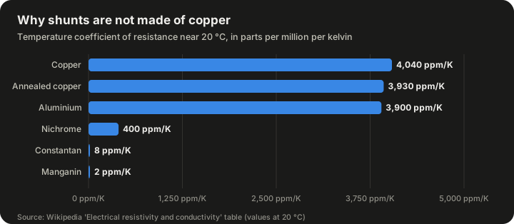
A shunt's resistance must stay constant as it warms up, or the measurement will drift with load. This is why shunts are made from special alloys rather than copper. The table below gives temperature coefficients of resistance near 20 °C from the reference table in the Wikipedia article on electrical resistivity and conductivity.
| Material | Resistivity at 20 °C (Ω·m) | Temperature coefficient (ppm/K) |
|---|---|---|
| Copper | 1.68 × 10⁻⁸ | 4,040 |
| Annealed copper | 1.72 × 10⁻⁸ | 3,930 |
| Aluminium | 2.82 × 10⁻⁸ | 3,900 |
| Nichrome | 110 × 10⁻⁸ | 400 |
| Constantan | 49.0 × 10⁻⁸ | 8 |
| Manganin | 48.2 × 10⁻⁸ | 2 |
Source: Wikipedia, "Electrical resistivity and conductivity," resistivity table at 20 °C (coefficients converted from K⁻¹ to ppm/K).
The difference is dramatic. Copper's resistance changes by about 0.4% for every kelvin of temperature change. Manganin's changes by about 0.0002%. A copper shunt that warms by 25 K under load would read about 10% high (4,040 ppm/K × 25 K ≈ 101,000 ppm ≈ 10.1%), while a manganin shunt under the same conditions would shift by about 50 ppm (2 ppm/K × 25 K), or 0.005%. This is the reason manganin and similar alloys dominate precision shunts.
Copper traces as sense resistors
Despite its temperature coefficient, copper is sometimes used deliberately. A section of printed circuit board trace has a small resistance and can serve as a "free" shunt, with no extra component and no extra cost. The Wikipedia article cites a Texas Instruments design note by L. Spaziani (1997), "Using Copper PCB Etch for Low Value Resistance," and work by Ziegler and colleagues (2008) who analysed the technique in detail. The drawbacks are that the signal is tiny, requiring a high-gain amplifier, and that accuracy is limited by trace manufacturing tolerance and copper's large temperature coefficient. A digital controller that knows the board temperature can correct for the drift, which Ziegler and colleagues showed is practical.
High-frequency and high-current shunts
At high frequencies, a shunt is no longer a pure resistance. Its parasitic inductance adds a voltage proportional to the rate of change of current, which corrupts fast measurements and causes errors at low power factor. Two historical developments addressed this:
- Skin-effect compensation. At high frequency, current crowds toward the surface of a conductor, changing its effective resistance. R. Malewski and colleagues published a method for eliminating skin-effect error in heavy-current shunts in the IEEE Transactions on Power Apparatus and Systems in 1981.
- The flat-strap sandwich shunt. F. Castelli introduced this design in the IEEE Transactions on Instrumentation and Measurement in 1999. It achieves similar frequency response and power loss to earlier designs but is cheaper and simpler to build.
Coaxial shunts, in which the current flows out along an inner tube and back along an outer one, cancel most of their own magnetic field and are used for fast, high-amplitude pulses.
Low-side and high-side placement
Where the shunt goes in the circuit matters. Texas Instruments' introductory series on current-sense amplifiers describes the two arrangements:
- Low-side sensing places the shunt between the load and ground. The voltage across it sits close to 0 V, so the amplifier's inputs must work at or near ground.
- High-side sensing places the shunt between the supply and the load. The amplifier must then tolerate a common-mode voltage equal to the supply voltage while measuring a difference of only millivolts. TI notes that many 24 V automotive applications require the current monitor to tolerate common-mode voltages up to 72 V.
Low-side sensing is simpler but disturbs the load's ground reference and cannot detect a short from the load to ground. High-side sensing avoids both problems at the cost of a more demanding amplifier.
Current transformers
How they work
A current transformer (CT) is a transformer whose primary is the conductor carrying the current to be measured, often a single straight bar or cable passed through a ring-shaped core. The secondary has many turns. By the transformer principle, the secondary current is a scaled-down copy of the primary current. A burden resistor across the secondary converts that current into a voltage for measurement.
The Wikipedia article on current transformers gives standard secondary ratings of 1 A and 5 A. A 4000:5 CT, for example, delivers 5 A on its secondary when 4,000 A flows in the primary, a ratio of 800 to 1.
CTs are passive, need no power supply and provide inherent isolation, which is why they are the workhorse of power-system metering and protection. They measure only AC, because a transformer responds to changing flux, not steady flux.
What limits CT accuracy
Bastos's lecture explains the CT's errors in terms of its equivalent circuit. Not all the primary current is transferred to the secondary: some is used to magnetise the core. This magnetising current causes both an amplitude (ratio) error and a phase error. To reduce it, designers maximise the core's magnetising inductance by using high-permeability materials such as silicon steel or nickel alloy, and minimise leakage inductance through good winding distribution.
The CT's low-frequency response is limited by the magnetising inductance, which causes "droop" when measuring pulses. Its high-frequency limit is set mainly by leakage inductance and stray capacitance. Bastos's comparison table puts typical CT bandwidth at 50 Hz up to a few hundred kilohertz, with ranges from tens of amps to tens of kiloamps and uncertainty typically not better than 1%.
Saturation is the other major limitation. A large DC component or a very large primary current can saturate the core, at which point the magnetising inductance collapses and the error grows sharply. The Wikipedia article defines the knee-point voltage as the point where a 10% rise in applied voltage causes a 50% rise in magnetising current. This matters most for protection CTs, which must stay accurate during faults of 20 to 30 times rated current. Metering CTs usually operate within 1.2 to 1.5 times rated current.
Accuracy classes
Because CTs are used for billing and protection, their accuracy is standardised. IEC 61869 (which replaced IEC 60044-1) and IEEE C57.13 are the two main standards. The IEC metering accuracy classes include 0.1, 0.2, 0.2S, 0.5, 0.5S, 1 and 3. The class number corresponds to the permitted ratio error at rated current: class 1 allows 1% and class 0.5 allows 0.5%. Each class also sets a maximum phase error. Protection CTs use classes such as 5P and 10P, where the number is the maximum composite error in percent at a stated multiple of rated current (the accuracy limit factor).
| Use | Example classes | What the class guarantees |
|---|---|---|
| Revenue metering | 0.2, 0.2S, 0.5, 0.5S | Small ratio and phase error over the normal load range |
| General metering | 1, 3 | Percent-level ratio error at rated current |
| Protection | 5P, 10P | Composite error within 5% or 10% up to a stated multiple of rated current |
Sources: Wikipedia, "Current transformer"; IEC 61869-2 class designations.
A safety warning
An important safety point: the secondary of a CT should never be opened while current flows in the primary. With no burden, the CT tries to drive its current into an effectively infinite impedance, and the secondary voltage can rise to dangerous levels. The Wikipedia article notes that for some CTs this can reach several kilovolts and cause arcing. Small CTs may be limited by core saturation, but fast transients can still induce hazardous voltages. Test switches on metering panels short the secondary before a meter is removed for this reason.
The Hereward transformer
In the 1960s, H. G. Hereward at CERN proposed an "active" current transformer that used electronic feedback to improve accuracy and extend low-frequency response. An amplifier senses the voltage across the burden and drives a compensation current that keeps the core flux at zero. Bastos explains that the effect is equivalent to multiplying the magnetising inductance by the amplifier's open-loop gain plus one. A CERN internal note by J. B. Sharp from 1962 describes the Hereward transformer as an induction-type beam monitor for the Proton Synchrotron. The idea of nulling core flux with feedback is the conceptual ancestor of the most accurate DC current sensors in use today.
Rogowski coils
Principle and history
A Rogowski coil is a helical coil of wire wound on a non-magnetic former, bent into a loop around the conductor being measured. Because it has no iron core, it cannot saturate. Its output voltage is proportional to the rate of change of the current, so an integrator is needed to recover a signal proportional to the current itself.
The Wikipedia article on the device records that Arthur Prince Chattock of Bristol described a similar instrument in 1887, but used it to measure magnetic fields. Walter Rogowski and W. Steinhaus gave the definitive description in 1912, and the coil is named after Rogowski.
The output of an ideal Rogowski coil, as given on that page, is
v(t) = −(A N μ₀ / l) × dI/dt
where A is the cross-sectional area of each turn, N the number of turns, l the length of the winding and μ₀ the magnetic constant (4π × 10⁻⁷ H/m).
Strengths and weaknesses
Rogowski coils have several practical advantages:
- They can be made flexible and open-ended, so they can be wrapped around a live conductor without disconnecting it.
- Their low inductance gives fast response. The Wikipedia article states response times down to several nanoseconds.
- They stay linear at very high currents because there is no core to saturate. Bastos's table lists high currents up to 100 kA as possible.
- There is no dangerous open-circuit condition, unlike a CT.
Their weaknesses mirror their strengths. Without a high-permeability core, sensitivity is low. The current sensing article notes that sensitivity can be raised with more turns or more integrator gain, but more turns increase self-capacitance and self-inductance (reducing bandwidth), and more gain requires an amplifier with higher gain-bandwidth product. Rogowski coils also cannot measure DC, because a steady current produces no changing flux. Flexible coils are sensitive to the position of the conductor inside the loop, with accuracy effects of 1% to 3% according to the Wikipedia article. Bastos's table gives typical uncertainty of a percent or so, with better performance possible using digital integrators, and bandwidth from a few hertz up to megahertz.
Typical applications include welding, arc furnaces, electromagnetic launchers, short-circuit testing of generators, harmonic measurement and lightning research.
The Hall effect and magnetic field sensors
The Hall effect
In 1879 the American physicist Edwin Hall discovered that when a current flows through a conductor in a magnetic field, a small voltage appears across the conductor at right angles to both the current and the field. The cause is the Lorentz force pushing moving charge carriers to one side. A Hall sensor exploits this: it measures the magnetic field produced by the current in a nearby conductor.
The signal is small. The Wikipedia article states that the Hall voltage is about 30 µV in a field of 1 gauss, which means a Hall current sensor needs a low-noise amplifier, temperature compensation and often a regulated supply. Below about 10 A, the field around a conductor is weak and comparable to the Earth's magnetic field, which creates gain, thermal and noise problems. Hall sensors measure AC, DC and pulsating current, and provide inherent isolation because they never touch the conductor.
Open-loop and closed-loop transducers
Most Hall current sensors use a magnetic core, a ring of soft magnetic material around the conductor, with a small air gap. The core concentrates the field into the gap, where the Hall element sits. There are two main designs, as Bastos describes:
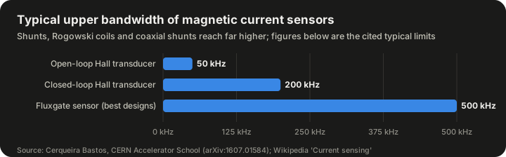
- Open-loop. The Hall voltage is simply amplified and becomes the output. This is cheap and simple. Bastos gives 1% uncertainty as typical and bandwidth typically not better than 50 kHz, with core geometry, lamination thickness, core material and the Hall chip all affecting the limit.
- Closed-loop (compensated). The Hall voltage drives a feedback amplifier that pushes current through a secondary winding on the core, cancelling the flux. The secondary current, an image of the primary, becomes the output. Because the core runs near zero flux, its nonlinearity and hysteresis matter much less. Bastos states that closed-loop devices are preferred for higher accuracy but are limited to no better than 0.1% uncertainty, with bandwidth up to 200 kHz.
Bastos summarises Hall transducers as "the transducers of choice for DC to AC current measurement applications, when percentage accuracy is required." They are cheap, simple, available in board-mounted and cable-mounted versions, and cover hundreds of milliamps to tens of kiloamps. Their accuracy limit comes mainly from the stability of the Hall element itself, which is affected by temperature and by mechanical stress (the piezoelectric effect).
Fluxgate sensors
A fluxgate sensor works like a closed-loop Hall sensor, but replaces the Hall element with a saturable inductor. The inductor is driven repeatedly in and out of saturation; any external field makes the saturation asymmetric, and this asymmetry is detected and nulled by feedback. The Wikipedia article lists the advantages as high resolution and accuracy, low offset and gain drift, and bandwidth up to 500 kHz in the best designs. The drawbacks are limited bandwidth in simpler designs, relatively high secondary power consumption, and the risk of injecting noise from the excitation back into the conductor being measured. The magnetic modulator principle on which fluxgates rely has been used since the 1930s in fluxgate magnetometers, according to Bastos.
| Sensor type | Typical upper bandwidth | Typical uncertainty |
|---|---|---|
| Open-loop Hall transducer | about 50 kHz | about 1% |
| Closed-loop Hall transducer | up to 200 kHz | no better than 0.1% |
| Fluxgate (best designs) | up to 500 kHz | high accuracy, low drift |
Source: Cerqueira Bastos, CERN Accelerator School (2014; arXiv:1607.01584) for Hall figures; Wikipedia, "Current sensing," for fluxgate bandwidth. Rogowski coils and coaxial shunts reach far higher bandwidths but are not shown.
Magnetoresistive sensors
Magnetoresistive sensors change their electrical resistance in response to a magnetic field. The family includes anisotropic magnetoresistance (AMR), giant magnetoresistance (GMR), giant magnetoimpedance (GMI) and tunnel magnetoresistance (TMR). They are usually arranged in a Wheatstone bridge to compensate for thermal drift. The Wikipedia article states that all of them are more sensitive than Hall sensors. GMR and TMR devices cost more than Hall devices and suffer from nonlinearity and thermal drift, and a strong external field can permanently change a GMR sensor's behaviour. GMI and TMR are more sensitive still and are in volume production from manufacturers including TDK, Crocus, Sensitec and MDT. Their higher sensitivity is especially attractive for small currents, where Hall sensors struggle with the weak field.
The zero-flux DCCT: the precision benchmark
Origins at CERN
The most accurate way to measure large DC currents is the zero-flux direct-current current transformer, usually called a DCCT. The Wikipedia article notes that it was introduced at CERN in the 1960s and is still regarded as the state of the art for high-accuracy current sensing. Bastos's lecture cites K. Unser's 1969 paper in the IEEE Transactions on Nuclear Science as the foundational reference for combining the Hereward feedback principle with the magnetic modulator to measure currents from DC to a few hundred kilohertz.
Bastos explains why accelerators drove this field: power converters for particle accelerators must deliver extremely accurate currents to the magnets that steer and focus the beam, and "a lot of the developments within the field of current measurement for power converters over the last 50 years have been driven by the accelerator community."
How a DCCT works
A DCCT's measuring head has three magnetic cores, all encircled by the primary conductor:
- Two matched cores are driven by a magnetic modulator in and out of saturation in opposite directions. If there is no net DC flux, the current peaks caused by saturation are symmetrical. If there is DC flux, they become unequal.
- The asymmetry is detected and measured.
- A third core picks up the AC component of the flux.
- A control loop combines the two signals and drives a compensation current through a secondary winding that makes the total flux zero.
The compensation current is a precise fractional image of the primary current. It flows through a burden resistor, and an amplifier measures the voltage. Because the cores operate at zero average flux, their nonlinearity largely drops out.
Where the errors come from
Bastos lists the main error sources:
- Magnetic head: sensitivity to external fields, to the return conductor, and to how well the primary is centred; magnetic remanence; modulation noise from imperfectly matched cores.
- Burden resistor: gain error, settling at full scale, stability, linearity and temperature coefficient. Bastos calls the burden resistor "the most common source of uncertainty in DCCTs."
- Output amplifier: offset error, settling and stability at zero, temperature coefficients, noise and common-mode rejection.
The burden resistor deserves special attention. Bastos explains that precision designs use four-wire resistors made with bulk metal foil, a rolled nickel-chromium foil bonded to an alumina substrate, engineered so that the foil's own temperature coefficient cancels the strain caused by the substrate's lower thermal expansion. The result is a near-zero coefficient for ambient temperature changes. But when the resistor heats itself, the temperature gradient is different and the effective coefficient turns negative, an effect described by the "power coefficient of resistance." Hysteresis under power cycling and moisture absorption also matter. Bastos makes the counter-intuitive point that tight tolerance and good stability do not always go together: processes that trim a resistor very precisely can create hot spots that degrade its stability.
How DCCTs compare
Bastos's comparison table puts DCCTs at the top of the accuracy ladder: the best devices reach parts-per-million uncertainty, they cover tens of amps to tens of kiloamps, and their bandwidth runs from DC up to a few hundred kilohertz for lower currents. They are also the most complex devices, with the most possible error sources.
| Device | Principle | Best uncertainty | Range | Bandwidth | Isolated? |
|---|---|---|---|---|---|
| DCCT | Zero-flux detector | ppm | tens of A to tens of kA | DC to a couple of hundred kHz | Yes |
| Hall transducer | Hall effect | 0.1% | hundreds of mA to tens of kA | DC to a couple of hundred kHz | Yes |
| Current transformer | Faraday's law | about 1% | tens of A to tens of kA | 50 Hz to a few hundred kHz | Yes |
| Rogowski coil | Faraday's law | percent level | up to 100 kA | a few Hz to MHz | Yes |
| Shunt | Ohm's law | ppm (low current) to percent (high current) | mA to several kA | up to hundreds of kHz (coaxial) | No |
Source: Cerqueira Bastos, "High Precision Current Measurement for Power Converters," CERN Accelerator School 2014, Table 1.
LHC-era developments
The Large Hadron Collider pushed DCCT performance further. Bastos cites work by G. Hudson and K. Bouwknegt (2005) on 4 to 13 kA DC current transducers designed for accurate in-situ calibration for the LHC, and work by P. Dreesen and colleagues (2007) characterising burden resistors for high-precision DCCTs. The Wikipedia article also cites a 2024 CERN report on the development of ultra-stable DCCTs for the High-Luminosity LHC power converters (CERN-OPEN-2024-006), showing the work continues.
Optical current sensors
The Faraday effect
When polarised light travels through a transparent material in a magnetic field aligned with its path, the plane of polarisation rotates. This is the Faraday effect. If an optical fibre is wound around a conductor, the total rotation is proportional to the current enclosed. An interferometer measures the resulting phase change. Because the sensing element is glass, it is inherently insulating, immune to electromagnetic interference and free of magnetic saturation.
An industrial example
ABB developed fibre-optic current sensors for DC measurement in the electrochemical and electrowinning industries, where aluminium, copper and chlorine plants run enormous direct currents through busbars. ABB's technical papers from around 2005 describe a sensor based on the Faraday effect in fused silica fibre, rated for 500 kA with a measuring range of ±600 kA (rated current plus 20% overcurrent). The papers report accuracy within ±0.1% over a wide range of currents and temperatures, and a later ABB article specifies 0.1% from 1% to 120% of rated current at temperatures from −40 to +80 °C. The fibre is packaged in a flexible strip that can be installed without opening the busbars. Because it has no magnetic yoke, it is smaller and lighter than an equivalent Hall-effect sensor. These figures are vendor-reported.
Fibre-optic sensors are also used in high-voltage substations, where the insulation advantage is decisive.
Clamp meters and other everyday tools
The most familiar current-sensing instrument for electricians is the clamp meter, which has jaws that open to surround a conductor. Older clamp meters are current transformers and measure only AC. Many modern ones use a Hall sensor or fluxgate in the jaw and can measure DC as well. The advantage is obvious: no wire has to be disconnected.
Digital multimeters, by contrast, usually measure current with an internal shunt, which is why the meter must be connected in series with the circuit and why its current input is protected by a fuse.
Turning current into data
Conditioning the signal
Almost every current sensor produces a signal that needs further processing:
- A shunt produces millivolts that must be amplified, often in the presence of a large common-mode voltage.
- A CT produces a current that must be converted to a voltage by a burden resistor.
- A Rogowski coil produces a derivative that must be integrated.
- A Hall element produces microvolts that must be amplified and temperature-compensated.
Dedicated current-sense amplifiers integrate the amplifier, gain-setting resistors and sometimes the analogue-to-digital converter in one package.
Digitisation and digital correction
Once digitised, the signal can be corrected in software. A copper-trace shunt can be compensated for temperature. A Rogowski coil can be integrated digitally, which Bastos notes can improve its accuracy. Gain and offset can be calibrated at the factory and stored. Bastos recommends digital calibration over potentiometer trimming in DCCT output stages, because a potentiometer upsets the matching of resistor ratios that sets common-mode rejection.
Isolation
Wherever the measured current is at a dangerous voltage, the measurement circuit must be isolated. Magnetic and optical sensors provide isolation by their nature. Shunts need an isolation amplifier, an isolated analogue-to-digital converter, or a digital isolator after conversion.
Testing and calibrating current sensors
At the precision end, how a sensor is tested matters as much as how it is built. Bastos describes four main test methods for DCCTs:
- Reference device method. The same primary current passes through the device under test and a reference device, and the readings are compared. Bastos notes that according to ANSI/NCSL Z540.3-2006, the reference must be at least four times better than the device under test.
- Reference current method. A small, accurately known current is injected into an auxiliary winding with enough turns to simulate the full primary ampere-turns. The DCCT output is measured with a precision voltmeter.
- Burden injection. A reference current is injected directly into the burden resistor in place of the compensation current. This isolates errors caused by the burden and output amplifier, but must be done carefully because of common-mode voltages.
- Back-to-back comparison. On current-output devices, a reference current is compared directly with the DCCT's output current.
Matching the strategy to the accuracy
Bastos also sets out how test and calibration effort should scale with the requirement:
| Application | Example requirement | Recommended approach |
|---|---|---|
| Very high accuracy | below 10 ppm relative accuracy, 50 ppm yearly drift | Individual testing of each unit in high-precision test beds; calibration winding method or reference units |
| Medium accuracy | below 100 ppm relative accuracy, 1,000 ppm yearly drift | Comparison against a reference unit; burden injection for field calibration |
| Low accuracy | percent-level yearly drift | Weigh calibration against cost; often no calibration |
Source: Cerqueira Bastos, CERN Accelerator School 2014, sections 3.7 and 3.8.
For the most demanding applications, Bastos lists the tests: centring, return-bar influence, external field influence, temperature coefficient, electromagnetic compatibility (voltage dips, burst immunity, conducted noise), gain, offset drift, settling at nominal current, linearity, noise, repeatability, reproducibility and settling at minimum current.
He also raises a practical question that is easy to overlook: what happens when a drifted sensor is replaced? In an accelerator, swapping a DCCT can cause a sudden jump in the current seen by the machine. Regular calibration limits the size of that jump.
How engineers choose a sensor
Bastos's selection guidance
For power-converter applications, Bastos offers a simple decision structure:
- High current, high accuracy (for example, above 1 kA and below 50 ppm): DCCTs are the devices of choice. These usually have a separate measuring head and electronics chassis, with the chassis installed close to the control electronics.
- Medium current, medium to high accuracy (hundreds of amps, below 100 ppm): DCCTs are still the only devices that deliver the required performance. Current-output versions can be an advantage when the electronics sit in a harsh environment far from the controller.
- Low accuracy (percent level): current transformers and Hall transducers are simpler and cheaper. Shunts are an option where isolation is not required.
- Fast applications: up to a few hundred kilohertz, the above still apply. Above that, Rogowski coils and coaxial shunts should be considered, as long as accuracy requirements stay around a percent.
A broader decision table
Combining the sources gives a general guide:
| If you need... | Consider... | Watch out for... |
|---|---|---|
| Cheapest possible DC and AC sensing on a board | Shunt with current-sense amplifier | Power loss, isolation, temperature drift |
| Isolated DC sensing at percent accuracy | Open-loop Hall | Offset drift, limited bandwidth |
| Isolated DC sensing at 0.1% | Closed-loop Hall or fluxgate | Power consumption, cost |
| ppm-level DC accuracy | Zero-flux DCCT | Complexity, burden resistor stability |
| AC metering or protection on the grid | Current transformer | Saturation, open-secondary hazard |
| Fast pulses or very large AC currents | Rogowski coil | No DC response, position sensitivity |
| Very large DC with high insulation | Fibre-optic sensor | Cost, specialist installation |
| Very small currents with isolation | Magnetoresistive (TMR, GMI) | Nonlinearity, external field damage |
A second worked example: open-loop Hall sensitivity (hypothetical)
Consider a hypothetical open-loop Hall sensor rated for 50 A full scale with a 1% typical uncertainty, the figure Bastos gives for open-loop devices.
- 1% of 50 A is 0.5 A.
- If the sensor is used to measure a 2 A standby current, an uncertainty of up to 0.5 A would be 25% of the reading.
This illustrates why full-scale specifications can be misleading at low currents, and why designers either choose a sensor rated close to the expected current or use a more accurate closed-loop design. It is also part of why Hall sensors become difficult below about 10 A, as the Wikipedia article notes.
Limits and practical problems
Every technology has failure modes that catch out designers.
Thermal effects. Shunts self-heat. Hall elements drift with temperature. Burden resistors in DCCTs change with self-heating. Thermoelectric voltages at junctions of dissimilar metals add offsets to millivolt-level shunt signals.
External magnetic fields. Every magnetic sensor responds to fields from sources other than the conductor of interest: neighbouring busbars, transformers, motors, even the Earth. Shielding, careful geometry and closed-loop designs reduce but do not eliminate this. Bastos notes that CTs and DCCTs both use magnetic shielding for this reason.
Saturation and remanence. Cored sensors can saturate under overload or large DC, and may retain magnetisation afterwards. The Wikipedia article notes that hysteresis can require demagnetisation to restore accuracy.
Bandwidth versus accuracy. The most accurate sensors (DCCTs) are limited to a few hundred kilohertz; the fastest (Rogowski coils, coaxial shunts) are limited to about a percent.
Electromagnetic interference. Switching power converters generate fast voltage edges that couple into sensor wiring. Bastos lists sensitivity to interference as a concern for Hall probes and includes EMC tests in DCCT qualification.
Noise injected into the primary. Fluxgates and DCCTs drive their cores with an excitation signal that can couple back into the circuit being measured. Bastos warns about modulation voltage noise and the voltage induced in the primary in fast applications.
Common misconceptions
"A current sensor measures current directly." Most don't. Shunts measure voltage, magnetic sensors measure field, and CTs measure an induced current. The current is always inferred through a physical law, and the accuracy depends on how well that law and its parameters hold.
"More expensive means more accurate." Not always for the job at hand. A ppm-level DCCT is useless for measuring nanosecond pulses, and a cheap shunt can outperform an expensive Hall sensor for low-frequency, low-voltage measurement.
"Copper is a good shunt material because it conducts well." High conductivity is exactly what you don't want, and copper's temperature coefficient is about 2,000 times larger than manganin's.
"A CT can measure DC if you're careful." A passive CT responds only to changing flux. DC also pushes the core towards saturation, degrading AC accuracy as well. Measuring DC requires an active technique such as a Hall sensor, fluxgate or DCCT.
"Rogowski coils are less accurate than CTs." Both are typically at the percent level in Bastos's comparison; the Rogowski coil trades a little sensitivity and DC response for freedom from saturation and much wider bandwidth.
"Accuracy on the datasheet is accuracy in my circuit." Datasheet figures assume specific conditions: temperature, conductor position, absence of external fields and a particular point in the range. Field accuracy is usually worse.
Applications across industries
Consumer electronics. Battery fuel gauges integrate current over time to estimate remaining charge. Chargers regulate current. Usually shunts with dedicated amplifiers or integrated sensing in power chips.
Automotive and electric vehicles. Battery management systems measure pack current for state of charge and safety, and inverters measure phase currents for motor control. Both shunts and Hall sensors are widely used, and high-side sensing is common, which is why automotive current monitors must tolerate high common-mode voltages.
Industrial drives. Variable-speed drives measure motor phase currents to control torque and detect faults. Closed-loop Hall transducers are a common choice because they combine isolation with good bandwidth.
Power grids. Current transformers dominate metering and protection, with fibre-optic sensors increasingly used at high voltage.
Heavy industry. Electrowinning and aluminium smelting run very large DC currents, where fibre-optic sensors and large DCCTs are used.
Science. Accelerator magnet power converters use DCCTs at the ppm level. Fusion and pulsed-power experiments use Rogowski coils for fast, enormous pulses.
Renewable energy. Solar inverters measure DC input current and AC output current, and must detect residual or leakage currents for safety.
Frequently asked questions
What is the most accurate way to measure DC current?
For large DC currents, the zero-flux DCCT, with best devices reaching parts-per-million uncertainty according to Bastos. For small currents where isolation is not needed, a precision shunt made from a low-temperature-coefficient alloy can also reach ppm-level uncertainty.
Can a Hall sensor measure AC?
Yes. Hall sensors measure the instantaneous magnetic field, so they follow both DC and AC. Their limit is bandwidth: Bastos gives about 50 kHz for typical open-loop devices and up to 200 kHz for closed-loop ones.
Why does a current transformer have a 1 A or 5 A secondary?
These are standard ratings that let meters and relays be built to a common input, regardless of the primary current. A 4000:5 CT and a 200:5 CT both deliver 5 A at their rated primary.
Why is it dangerous to open a CT's secondary?
With no burden, the CT tries to force its current through an infinite impedance, and the secondary voltage can climb to dangerous levels, in some cases several kilovolts.
Can a Rogowski coil measure DC?
No. Its output depends on the rate of change of current, and a steady current produces no output.
What is a sense resistor?
A low-value resistor placed in series with a load so that the voltage across it indicates the current. "Shunt" and "sense resistor" are generally used for the same thing.
What is the difference between high-side and low-side sensing?
Low-side places the shunt between the load and ground; high-side places it between the supply and the load. High-side sensing needs an amplifier that tolerates the supply voltage as a common-mode voltage but keeps the load's ground intact.
Why does a precision current sensor need calibrating?
Because components drift. Bastos gives examples of yearly drift requirements from 50 ppm to 1,000 ppm, depending on the application. Calibration tracks the drift and, in systems with many converters, keeps them consistent with each other.
A short history
| Year | Development |
|---|---|
| 1879 | Edwin Hall discovers the Hall effect |
| 1887 | A. P. Chattock describes a coil similar to the Rogowski coil, used for magnetic fields |
| 1912 | Walter Rogowski and W. Steinhaus publish the definitive description of the Rogowski coil |
| 1930s | Magnetic modulator principle in use in fluxgate magnetometers |
| 1960s | H. G. Hereward proposes the active, flux-nulling current transformer at CERN (1962 CERN note by J. B. Sharp) |
| 1969 | K. Unser publishes on the DC current transformer in IEEE Transactions on Nuclear Science |
| 1981 | Malewski and colleagues publish skin-effect error elimination for heavy-current shunts |
| 1997 | Spaziani's TI design note on PCB copper as a sense resistor |
| 1999 | Castelli introduces the flat-strap sandwich shunt |
| 2001 | Costa and colleagues publish "The Current Sensors in Power Electronics, a Review" in the EPE Journal |
| 2005 | ABB describes 500 kA-rated fibre-optic DC current sensors for electrowinning; Hudson and Bouwknegt describe 4 to 13 kA DCCTs for the LHC |
| 2009 | Ziegler and colleagues publish "Current Sensing Techniques: A Review" in IEEE Sensors Journal |
| 2024 | CERN reports on ultra-stable DCCTs for the High-Luminosity LHC |
Summary
Current sensing is a set of trade-offs rather than a single technology. Shunts are cheap and accurate but waste power and offer no isolation. Current transformers are robust and isolating but measure only AC and can saturate. Rogowski coils are fast, flexible and unsaturable but cannot see DC. Hall-effect sensors measure DC and AC with isolation at percent or tenth-of-a-percent accuracy. Fluxgates and magnetoresistive sensors improve sensitivity and drift. Fibre-optic sensors handle huge DC currents at high voltage. At the top of the accuracy ladder, the zero-flux DCCT, developed in the accelerator community from the 1960s onward, reaches parts-per-million uncertainty. Choosing well means starting from the requirement (current range, accuracy, bandwidth, isolation, cost) and accepting the weaknesses of the technology that best fits it.
Sources
- Current sensing (Wikipedia)
- Cerqueira Bastos, M. High Precision Current Measurement for Power Converters. CERN Accelerator School 2014 (arXiv:1607.01584)
- Current transformer (Wikipedia)
- Rogowski coil (Wikipedia)
- Electrical resistivity and conductivity (Wikipedia)
- How to Get Started with Current Sense Amplifiers, Part 1 (Texas Instruments, 2015)
- Fiber-optic DC current sensor for the electrowinning industry (ABB)
- Light Measures Current (T&D World)
- IEC 61869-2 information preview (VDE Verlag)