A black-box model of a power converter describes how a converter behaves at its terminals without describing what happens inside it. The converter might be a laptop charger, a motor drive, a server power supply, or a DC-DC module on an aircraft. Whatever it is, the black-box approach treats it as a sealed box with a few wires coming out. The model is built from measurements (or simulations) taken at those wires, and it answers practical questions: how much electrical noise will this box push back into the supply, how will it react when a filter or a cable is connected to it, and will it stay stable when it is plugged into a particular source?
The idea comes from system identification, the branch of engineering that builds mathematical models of systems from observed inputs and outputs. In power electronics it has two main uses. The first, and the one the Wikipedia article on the subject concentrates on, is electromagnetic compatibility (EMC): predicting the conducted noise a switching converter produces and designing the filter that keeps that noise within legal limits. The second is system-level simulation and stability analysis of power distribution networks, where many converters made by different vendors must work together on a shared bus.
This article explains why such models are needed, how they are built, what assumptions they rest on, how the passive parts of the model are measured, what the research literature has actually demonstrated, and where the method breaks down.
Why model a converter as a black box at all?
Switching converters are noisy by design
A modern switch-mode power supply (SMPS) converts power by turning semiconductor switches fully on and fully off, many thousands or millions of times per second. This is efficient, because a switch that is fully on or fully off dissipates little power, but it creates sharp edges in voltage and current. Those edges contain energy spread across a wide band of frequencies, and some of that energy escapes onto the power cables as conducted electromagnetic interference (EMI). Left unchecked, it can disturb radio reception and other equipment sharing the supply.
Regulators therefore set limits on how much high-frequency voltage a product may put back onto the mains. In the United States the rule for unintentional radiators such as computers and power supplies is 47 CFR §15.107, which limits the radio-frequency voltage conducted back onto the AC power line between 150 kHz and 30 MHz, measured through a 50 µH/50 Ω line impedance stabilization network (LISN). Internationally, the corresponding product standard for multimedia and information technology equipment is CISPR 32 (published in Europe as EN 55032), whose Class B mains limits match the US Class B figures.
The chart: what the limits look like
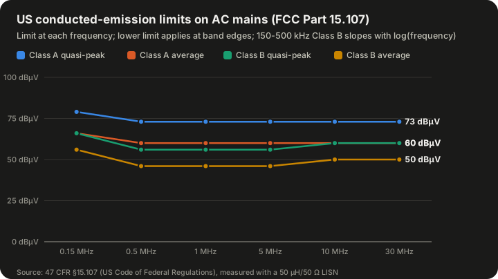
| Frequency band | Class A quasi-peak (dBµV) | Class A average (dBµV) | Class B quasi-peak (dBµV) | Class B average (dBµV) |
|---|---|---|---|---|
| 0.15–0.5 MHz | 79 | 66 | 66 falling to 56 | 56 falling to 46 |
| 0.5–5 MHz | 73 | 60 | 56 | 46 |
| 5–30 MHz | 73 | 60 | 60 | 50 |
Source: 47 CFR §15.107. In the 0.15–0.5 MHz band the Class B limits decrease with the logarithm of frequency; the lower limit applies at band edges.
Class B limits apply to equipment marketed for residential use and are tighter than Class A limits, which apply to commercial and industrial equipment. The difference between the two is 13 dB in the lowest band for the quasi-peak detector (79 versus 66 dBµV), which is a factor of about 4.5 in voltage.
Why a model is needed before the hardware is final
Meeting these limits almost always requires an EMI filter between the converter and the mains: inductors, capacitors and often a common-mode choke. The filter's job is to attenuate the noise by enough decibels at every frequency in the band. The trouble is that a filter's attenuation is not a fixed property of the filter. It depends on the impedances on both sides of it: the impedance of the source (here, the noisy converter) and the impedance of the load (the LISN or the real mains network).
Filter datasheets usually quote insertion loss measured in a 50 Ω system, with 50 Ω on both sides. A switching converter is not a 50 Ω source. Its noise source impedance can be much higher or much lower than 50 Ω, and it changes with frequency. Baisden's 2009 Virginia Tech dissertation reports that a black-box terminal model predicted filter attenuation more accurately than network-analyzer insertion-gain measurements, which is exactly the problem in a nutshell: a filter that looks good on a datasheet can underperform once it is connected to the real converter.
So an engineer wants two things about the converter: the noise it generates, and the impedance through which that noise is presented to the outside world. That pair is precisely what a black-box model supplies.
Why not just model the inside?
A detailed internal model, often called a white-box model, would include every switch, diode, magnetic component, capacitor, parasitic inductance of the circuit board traces and stray capacitance from the switch to the heat sink. Such models are possible and are used in research, but they have drawbacks:
- They require knowledge of the internal design, which a system integrator buying a converter from a supplier usually does not have.
- Parasitic elements, which dominate behaviour in the megahertz range, are hard to estimate accurately.
- Detailed switching simulations are slow, because they must resolve nanosecond edges across many switching cycles.
A black-box model sidesteps all three. It needs no schematic, it captures the real parasitics because it is built from measurements of the real unit, and once built it is a small linear circuit that solves quickly.
Terminology: white, grey and black boxes
The colour vocabulary is borrowed from system identification and is used loosely in practice.
| Model type | What it uses | Typical strengths | Typical weaknesses |
|---|---|---|---|
| White box | Full internal circuit, component values, parasitics, control law | Physical insight; can predict effect of design changes | Needs design data; parasitics hard to know; slow to simulate |
| Grey box | A chosen structure based on physics, with parameters fitted from measurements | Fewer parameters; some physical meaning retained | Structure must be guessed correctly |
| Black box | Only terminal voltages and currents, measured or simulated | No internal knowledge needed; includes real parasitics | Valid only near the conditions measured; little physical insight |
The power-converter black-box model sits at the black end of this scale, though, as discussed below, the choice of an equivalent-circuit structure with sources and impedances does impose some physical assumptions.
What the model looks like
Terminated and unterminated models
The Wikipedia article distinguishes two forms:
- A terminated model includes the load. The converter and whatever it is driving are characterised together as one box.
- An unterminated model excludes the load, so it describes the converter alone and can be connected to different loads in simulation.
The distinction matters because the noise a converter produces at its input depends partly on what is connected to its output. A terminated model is simpler to build but valid only for that load; an unterminated model is more general but needs more measurement effort.
The same terminology appears in the stability-oriented literature. Luis Arnedo's 2008 Virginia Tech dissertation, "System Level Black-Box Models for DC-DC Converters", builds its models from what it calls unterminated frequency response measurements: quantities such as input admittance, output impedance, audio-susceptibility and back-current gain, measured so that they contain no information about the dynamics of the particular source or load used during testing.
Active and passive parts
In the EMI form described in the Wikipedia article, the equivalent circuit is defined in the frequency domain and contains two kinds of elements:
- Active components: at least two sources, which may be two voltage sources, two current sources, or one of each. These represent the noise generated by the switching action.
- Passive components: impedances or admittances, or more generally a two-port network described by an impedance (Z) matrix or admittance (Y) matrix. These represent how the converter's internal paths present that noise to the terminals.
At each frequency, the sources are complex numbers (an amplitude and a phase) and the impedances are complex numbers. Because the model is in the frequency domain, a separate set of values exists for every frequency of interest; in practice they are stored as tables across the EMI band.
Why two sources?
Conducted noise on a pair of power lines has two components:
- Differential-mode (DM) noise flows out on one line and back on the other, like the normal power current. It is driven mainly by the pulsating input current of the converter.
- Common-mode (CM) noise flows out on both lines together and returns through the ground or chassis, often via stray capacitance between a switching node and the grounded heat sink.
The two modes travel by different paths, see different impedances, and are attenuated by different parts of a filter (DM by line-to-line capacitors and DM inductance, CM by line-to-ground capacitors and the common-mode choke). A model that represents both needs at least two independent sources, one for each mode or one for each line with respect to ground.
Thevenin and Norton forms
The simplest building block of these models is familiar from introductory circuit theory. Any linear one-port network, at a given frequency, can be replaced by either:
- a Thevenin equivalent: a voltage source in series with an impedance, or
- a Norton equivalent: a current source in parallel with an impedance.
The black-box EMI model is essentially the multi-terminal extension of this idea. Where a two-wire DC input has three terminals (positive, negative and ground), the model needs a source and an impedance structure that can reproduce the voltages and currents at all of them.
The Wikipedia article notes that six equivalent circuit types are in use. They differ in whether the sources are voltage or current sources and in how the impedances are arranged (for example as a star or a delta of three impedances). Mathematically they are interchangeable: a star of impedances can be converted into a delta, and a Thevenin source into a Norton source. The choice is usually made for measurement convenience.
The core assumptions
The model rests on two assumptions, and the Wikipedia article is candid about both.
Assumption 1: linearity
A switching converter is fundamentally nonlinear and time-variant. Its switches change state, its diodes conduct only part of each cycle, and its magnetic cores may approach saturation. Sounitro Banerjee's book on nonlinear phenomena in power electronics (Wiley, 2001) is one of the standard references on just how rich that nonlinear behaviour can be, including bifurcations and chaos.
For EMI purposes, though, the model treats the noise as a small signal superimposed on the converter's normal operation. As long as the filter is designed so that its components do not saturate and nonlinear effects are avoided, the relationship between the noise sources and the terminal voltages can be treated as linear. That is what allows the use of superposition, impedances and Kirchhoff's laws.
Assumption 2: invariance
The equivalent circuit is assumed to be the same across the operating conditions used to identify it. This sounds obvious, but it is a strong statement. To identify the model, the engineer deliberately changes the external impedance connected to the converter, and assumes that this change alters only the external circuit, not the noise sources or internal impedances themselves.
In reality, changing the external impedance can shift switching transitions slightly, or alter the converter's operating point. The model works when those shifts are small. Baisden's dissertation addresses the problem for systems whose operating point varies, such as converters fed from or feeding AC systems, where the internal state changes throughout each line cycle; it uses simplification techniques to keep the amount of data manageable.
How the model is identified: a worked example of the method
The counting argument
The Wikipedia article gives a compact example of how the model's unknowns are found. Suppose the chosen equivalent circuit has three impedances and two current sources. That is five unknowns at each frequency.
The engineer creates three operating conditions by changing the external impedance connected to the converter's terminals. In each condition, the terminal voltages and currents are measured (or simulated). Applying Kirchhoff's circuit laws and nodal analysis to each condition gives two independent equations, so three conditions give six equations. Six equations for five unknowns is enough to solve the system, with one equation to spare as a check or to reduce the effect of measurement error.
The same process is repeated at every frequency of interest, producing frequency-dependent tables for each source and impedance.
A simple hypothetical one-port example
The arithmetic is easier to see with a simpler model: a single Thevenin source and a single impedance. The following is a hypothetical example with round numbers, using real (resistive) values for clarity. In a real measurement, every quantity is complex and the arithmetic is done with magnitudes and phases.
At one frequency, suppose the converter's noise voltage is measured across two different external loads:
| Condition | External load Z_L | Measured terminal noise voltage V |
|---|---|---|
| 1 | 50 Ω | 2.0 mV |
| 2 | 10 Ω | 1.0 mV |
For a Thevenin source V_s with internal impedance Z_s, the terminal voltage is a voltage divider:
V = V_s × Z_L / (Z_s + Z_L)
Writing this for both conditions:
- 2.0 × (Z_s + 50) = 50 × V_s
- 1.0 × (Z_s + 10) = 10 × V_s
From the second equation, V_s = (Z_s + 10) / 10. Substituting into the first: 2Z_s + 100 = 5Z_s + 50, so 3Z_s = 50 and Z_s ≈ 16.7 Ω. Then V_s = 26.7 / 10 ≈ 2.67 mV.
Checking: with a 50 Ω load, 2.67 × 50 / 66.7 ≈ 2.0 mV; with a 10 Ω load, 2.67 × 10 / 26.7 ≈ 1.0 mV. Both match.
The useful result is that the model now predicts the noise for any load at that frequency, including a filter that has not been built yet. That is the whole point of the black-box approach: two or three measurements replace an unbounded number of trial-and-error filter builds.
Converting to decibels
EMI limits are expressed in dBµV, decibels relative to one microvolt:
dBµV = 20 × log10(V / 1 µV)
So 2.0 mV is 2,000 µV, which is 20 × log10(2000) ≈ 66.0 dBµV. Continuing the hypothetical, if this voltage appeared across a 50 Ω LISN at 1 MHz, it would sit about 10 dB above the Class B quasi-peak limit of 56 dBµV for that band. The engineer would then design a filter whose attenuation, computed using the model's source impedance rather than an assumed 50 Ω, exceeds 10 dB at that frequency by whatever margin the project requires.
Measuring the passive elements
The sources can be inferred from terminal measurements during operation, but the impedances are often measured directly. The Wikipedia article describes three methods, and each has its own trade-offs.
Method 1: converter switched off
The conventional approach is to switch the converter off and measure the impedance between its terminals with an impedance analyzer, or to measure scattering parameters (S-parameters) with a vector network analyzer (VNA) and convert them to impedance.
This is simple and uses standard laboratory instruments, but it assumes that the impedance is the same when the converter is off as when it is running. That assumption is questionable. When the converter is running, semiconductors are conducting or blocking, diodes are switching, and magnetic components carry current that changes their permeability. An unpowered converter can present a different impedance from a working one.
Method 2: clamp-on current probes during operation
To measure impedance while the converter is running, Vuttipon Tarateeraseth, Bo Hu, Kye Yak See and Flavio Canavero published a method in IEEE Transactions on Power Electronics in 2010 ("Accurate Extraction of Noise Source Impedance of an SMPS Under Operating Conditions", vol. 25, no. 1, pp. 111–117).
The setup uses two clamp-on current probes connected to a VNA: one probe injects a test signal into the power wiring, and the other receives the resulting current. Because the probes clamp around the wires, there is no direct electrical contact with the power lines between the LISN and the power supply, so the measurement equipment is isolated from the mains voltage. After a calibration step that removes the effect of the probes and the wiring, both the common-mode and differential-mode noise source impedances can be extracted.
The method was developed partly to overcome weaknesses of earlier approaches. Insertion-loss methods depended on assumptions about component impedances, and resonance methods gave only the magnitude of the impedance, with phase information recoverable only through a complicated Hilbert-transform process. The Wikipedia article notes that the calibration for the clamp-on method is delicate: small errors in characterising the probes and the loop translate directly into errors in the extracted impedance.
Method 3: transformer coupling with an impedance analyzer
A third approach, associated with Mazzola, Grassi and Amaducci's work in IEEE Transactions on Electromagnetic Compatibility ("Novel Measurement Procedure for Switched-Mode Power Supply Modal Impedances", vol. 62, no. 4, pp. 1349–1357), uses transformers to couple an impedance analyzer to the running converter. Two setups are used, one to measure common-mode impedance and one for differential-mode impedance.
The transformer isolates the analyzer from the converter's operating voltage, which is the main obstacle to using an impedance analyzer on live equipment. The limitation, as the Wikipedia article notes, is that the usable measurement range is limited by the transformer's own frequency response and coupling.
Comparing the methods
| Method | Converter state | Main advantage | Main limitation |
|---|---|---|---|
| Impedance analyzer or VNA, unit off | Off | Simple; standard equipment | Assumes off-state impedance equals operating impedance |
| Two clamp-on probes with VNA | Operating | No galvanic contact; CM and DM both extracted | Delicate calibration |
| Transformer-coupled impedance analyzer | Operating | Analyzer isolated from mains | Range limited by the transformer |
What the research has demonstrated
Much of the systematic work on black-box EMI terminal models came from the Center for Power Electronics Systems (CPES) at Virginia Tech, under Dushan Boroyevich and colleagues.
Baisden's generalized terminal model
Andrew Carson Baisden's 2009 PhD dissertation, "Generalized Terminal Modeling of Electro-Magnetic Interference" (Virginia Tech, committee chair Dushan Boroyevich), proposed two- and three-terminal black-box models for EMI characterisation. The models are linear equivalent circuits in the frequency domain, with impedances and sources representing the noise across the EMI spectrum. The method was verified on a DC-DC boost converter, a phase-leg module and a simulated DC-AC inverter. Accuracy was confirmed up to 100 MHz in simulation and to at least 50 MHz experimentally.
The three-terminal version was published by Baisden, Boroyevich and Fei Wang in IEEE Transactions on Industry Applications in 2010 (vol. 46, no. 5, pp. 2068–2079), building a linearised equivalent circuit of a power electronic system at a given operating point and confirming its accuracy up to 100 MHz for a DC-DC boost converter.
Extensions to inverters and buck-type inputs
Hemant Bishnoi, Baisden, Paolo Mattavelli and Boroyevich applied the approach to a DC-AC half-bridge inverter at the 2011 IEEE Applied Power Electronics Conference (APEC), reporting measured and predicted emissions in good agreement, within 6 dB, up to 30 MHz. Their 2012 paper in IEEE Transactions on Power Electronics ("Analysis of EMI Terminal Modeling of Switched Power Converters", vol. 27, no. 9, pp. 3924–3933) extended the technique to converters with buck-type inputs, with predictions up to 100 MHz and errors of 6 dB or less at most frequencies. The work was aimed partly at aerospace applications, where EMI limits are strict.
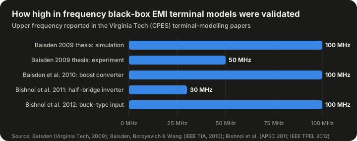
| Study | System | Validated up to |
|---|---|---|
| Baisden 2009 dissertation (simulation) | Boost converter, phase-leg, inverter | 100 MHz |
| Baisden 2009 dissertation (experiment) | Hardware tests | at least 50 MHz |
| Baisden, Boroyevich and Wang 2010 | DC-DC boost converter | 100 MHz |
| Bishnoi et al. 2011 (APEC) | DC-AC half-bridge inverter | 30 MHz, within 6 dB |
| Bishnoi et al. 2012 (IEEE TPEL) | Buck-type input converters | 100 MHz, 6 dB or less at most frequencies |
Source: Virginia Tech VTechWorks record of Baisden (2009); IEEE abstracts of Baisden et al. (2010) and Bishnoi et al. (2011, 2012).
Two points are worth drawing out. First, the regulatory conducted band ends at 30 MHz, so models validated to 50 or 100 MHz cover it with room to spare; higher frequencies matter for radiated emissions and for understanding filter parasitics. Second, an accuracy of "within 6 dB" means the predicted voltage can be off by up to a factor of two. That is respectable for EMI work, where emissions span many tens of decibels and test-to-test repeatability is itself limited, but it is not precision measurement. Designers still leave margin.
A note of caution about sources: a 2014 conference paper with the same title as the 2012 Bishnoi paper was flagged by IEEE with a notice of violation of its publication principles. Readers following the literature should cite the 2012 Transactions paper.
The other family: black-box models for system stability
The problem of interconnected converters
The second main use of black-box converter models is not EMI but stability. Spacecraft, aircraft, ships, data centres and electric vehicles increasingly distribute power on DC buses that feed many converters. A converter that regulates its output tightly draws constant power from its input. If its input voltage rises, its input current falls, and vice versa. Over the converter's control bandwidth, it therefore looks like a negative incremental resistance.
For an ideal constant-power load drawing power P from a voltage V, the incremental input resistance is:
R_in = −V² / P
As a hypothetical example, a 100 W converter on a 48 V bus presents R_in = −(48 × 48) / 100 = −23.04 Ω at low frequency. A negative resistance can cancel the positive damping of an input filter's resistance and turn the combination into an oscillator.
Middlebrook's criterion
The classic treatment is R. David Middlebrook's 1976 paper "Input Filter Considerations in Design and Application of Switching Regulators", presented at the IEEE Industry Applications Society annual meeting. Middlebrook, a Caltech professor, set out what is often called the Middlebrook criterion: the output impedance of the source or input filter should be small compared with the input impedance of the converter across frequency. Secondary sources describe it as a sufficient but not necessary condition for stability, which makes it conservative but convenient, because it depends only on impedance magnitudes, quantities that can be measured at the terminals.
This is where the black-box idea comes in. The criterion needs only terminal impedances, not internal details, so a black-box model of each converter is enough to check whether a proposed system will be stable.
Arnedo's system-level models
Arnedo's 2008 dissertation developed black-box models of two-port DC-DC converters for system-level simulation. The models need no internal circuit, structure or control details. They are identified from unterminated frequency response measurements at the power terminals, and the author showed how source and load effects can be separated from measurements made with real sources and loads.
A single linear model only holds near one operating point, so the work combined families of linear models into two structures:
- A Wiener structure, suitable when the converter's nonlinearity shows up mainly in its steady-state currents and voltages.
- A polytopic structure, which blends several linear models with weighting functions and handles nonlinearity that affects transient behaviour as well.
The dissertation validated simulation and stability results against experimental data for converters from two different manufacturers. Arnedo and colleagues also presented unterminated measurement and model-order reduction methods at APEC in 2008, and later work on polytopic models with dynamic weighting functions appeared in IEEE Access in 2019.
EMI models versus stability models
| Aspect | EMI black-box model | Stability (system-level) black-box model |
|---|---|---|
| Frequency range | About 150 kHz to tens of MHz | DC to the control bandwidth (typically far below the switching frequency) |
| What the sources represent | Switching noise | Not noise; the model represents averaged dynamic response |
| Key quantities | Noise source amplitudes, CM/DM impedances | Input admittance, output impedance, audio-susceptibility, back-current gain |
| Typical question | Will the product pass the conducted emissions test with this filter? | Will this bus with these converters oscillate? |
| Nonlinearity handling | Linear at an operating point | Wiener or polytopic combinations of linear models |
Both families share the same philosophy: describe the box only by what can be observed at its terminals, and accept validity limited to the conditions identified.
Using the model to design an EMI filter
The workflow
A typical design flow using a black-box EMI model looks like this:
- Characterise the converter. Measure terminal voltages and currents under several external impedance conditions, or measure the impedances directly with one of the methods above, at frequencies covering the band of interest.
- Extract the model. Solve for the sources and impedances at each frequency.
- Build the system model. Connect the converter model to models of the LISN (or real network), cables and a candidate filter.
- Predict emissions. Calculate the noise voltage at the LISN measurement port and compare with the limit line, separately for CM and DM where needed.
- Iterate the filter. Adjust filter components in simulation until the prediction meets the limit with margin.
- Verify. Build the filter and confirm with a real compliance or pre-compliance measurement.
Why source impedance changes filter performance
A filter attenuates by creating an impedance mismatch: a series inductor works best when it faces a low source impedance and a low load impedance, because its own impedance then dominates the current path; a shunt capacitor works best when it faces high impedances, because it then diverts most of the noise current. If the converter's noise source impedance is low at a frequency where the filter designer assumed it was high, a shunt capacitor at the converter side does little. The model reveals this before hardware is built.
This is also why simple insertion-loss data can mislead. Insertion loss measured with 50 Ω on both sides tells you how the filter behaves between two 50 Ω ports; it does not tell you how the filter behaves between a converter with, say, a few ohms of DM impedance and a LISN.
Separating common and differential modes
Because filter components act on different modes, practical models usually express the noise in modal form. Common-mode noise is reduced mainly by the common-mode choke and line-to-ground (Y) capacitors; differential-mode noise is reduced by line-to-line (X) capacitors and the leakage inductance of the choke or separate DM inductors. Both the clamp-on probe method and the transformer method are designed to measure CM and DM impedances separately for this reason.
There is a further subtlety: in real circuits the two modes can convert into each other if the circuit is unbalanced, for example if the two lines have different stray capacitances to ground. A model that represents the three terminals with a full matrix of impedances can capture this mixed-mode behaviour, which is one reason the three-terminal models in the Baisden work use a more general network than a simple pair of independent modal sources.
Limits of the black-box approach
Validity is local
Every black-box model is valid only near the conditions under which it was identified. If the converter's input voltage, output load, temperature or switching frequency changes significantly, the noise sources and impedances may change too. Converters with frequency-hopping or spread-spectrum modulation, light-load burst modes or variable-frequency control can present a different noise spectrum at each operating point. A model identified at full load can underpredict emissions at light load, or vice versa. The practical response is to identify models at several operating points, which is what the polytopic and Wiener approaches do for stability work and what Baisden's simplification techniques do for time-varying operating points.
The linearity assumption can fail
If a filter inductor saturates, or if the filter alters the converter's switching transitions, the linear superposition assumed by the model no longer holds. The Wikipedia article's statement of the linearity assumption carries this condition explicitly: it applies when the filter is designed to avoid saturation and nonlinear effects.
Measurement difficulty
Measuring impedance on an operating converter is hard. The converter is connected to mains or a high-voltage bus, its own noise contaminates the measurement signal, and the probes or transformers used to isolate the instrument have their own frequency-dependent behaviour that must be calibrated out. Small calibration errors can lead to large errors in extracted impedance, especially when the converter impedance is very high or very low relative to the measurement system.
Little design insight
A black-box model tells you what the converter does at its terminals, not why. If the model shows a large common-mode source at 12 MHz, it cannot tell you whether the cause is the heat-sink capacitance, the transformer interwinding capacitance or the layout of a particular trace. For diagnosing and fixing noise at the source, white-box or grey-box modelling, near-field probing and layout inspection remain necessary.
Accuracy is moderate
The published validation results show agreement to within about 6 dB over most of the band. That is good for system-level design and filter sizing, but the final verdict on compliance still comes from a formal measurement on a real unit in a real test setup.
Common misconceptions
"A black-box model is just a measurement." It is more than that. A single emissions measurement tells you the noise for one setup. A black-box model separates the noise source from the impedance, so it predicts the noise for setups that have not been measured.
"If the filter has 60 dB of insertion loss, it will give 60 dB of attenuation." Only if the source and load impedances match the conditions under which the insertion loss was measured, typically 50 Ω on both sides. With a real converter, the attenuation can be considerably different, and the black-box model exists partly to quantify that difference.
"Switching converters are nonlinear, so linear models are wrong." The converter's large-signal behaviour is nonlinear, but the noise behaviour around a fixed operating point can be represented linearly, provided the filter and connected circuits stay linear. This is the same trick used throughout electronics, where small-signal models describe transistors that are fundamentally nonlinear devices.
"Unpowered impedance measurements are good enough." Sometimes they are, but they rest on the assumption that the off-state impedance equals the on-state impedance. The clamp-on probe and transformer methods were developed precisely because that assumption is not always safe.
"Black-box models replace compliance testing." They do not. They reduce the number of design iterations and help avoid failed tests, but legal compliance is determined by standardised measurement on the product.
A short history
The ingredients of the black-box converter model are old. Thevenin's and Norton's theorems, which underpin the equivalent circuits, date from the late nineteenth and early twentieth centuries. Two-port network theory, with its Z and Y matrices, is a standard part of circuit theory. System identification as a discipline grew from control engineering in the mid-twentieth century.
In power electronics specifically, the stability thread can be traced to Middlebrook's 1976 input filter paper, which established the practice of reasoning about converter interactions through terminal impedances. The EMI thread grew as switching converters became ubiquitous and regulatory limits such as the FCC Part 15 rules and the CISPR standards forced designers to predict and control conducted noise.
The two strands converged at Virginia Tech's CPES in the 2000s and early 2010s, where Arnedo's 2008 dissertation developed black-box models for system-level DC-DC simulation and stability, and Baisden's 2009 dissertation, followed by the 2010 and 2012 journal papers, developed generalised terminal models for EMI. In parallel, measurement researchers including Tarateeraseth, See, Canavero and colleagues improved methods for extracting noise source impedance under operating conditions (2010), and later Mazzola, Grassi and Amaducci proposed further procedures for SMPS modal impedance measurement.
More recently, black-box methods have been applied to grid-connected inverters, where small-signal impedance models of inverters identified from terminal measurements are used to assess interactions with weak grids. The underlying logic is unchanged: identify the box from its terminals and use the result to predict how it behaves in a larger system.
Applications
Product EMI design
The most direct use is designing input filters for power supplies, motor drives and inverters to meet conducted emission limits. The model lets a designer evaluate filter topologies and component values in simulation before committing to hardware.
System integration with purchased modules
System integrators often buy DC-DC modules or power supplies from vendors who will not release schematics. A black-box model built from the integrator's own measurements allows filter and bus design without internal information.
Aerospace and defence power systems
Aircraft and spacecraft power buses have strict EMI requirements and many interconnected converters. The Bishnoi 2012 work explicitly targeted aerospace applications. Stability of such buses is also critical, which makes the Arnedo-type stability models relevant.
DC distribution systems
Data centres, ships, microgrids and electric vehicles distribute DC power to many loads. Black-box models of each converter allow system designers to check interactions and stability using measured terminal behaviour.
Teaching and pre-compliance
Because the model reduces to a small linear circuit, it is also a useful teaching tool for showing why filters behave differently from datasheet expectations and how CM and DM noise paths differ.
Frequently asked questions
Is a black-box model the same as a behavioural model?
They overlap. "Behavioural model" is a broad term for any model that reproduces external behaviour without detailed internal physics. A black-box terminal model is one specific kind, built from terminal measurements and expressed as sources and impedances or as two-port network parameters.
What frequency range does an EMI black-box model need to cover?
For conducted emissions under the FCC and CISPR rules discussed above, 150 kHz to 30 MHz. The research models discussed here were validated up to 50 or 100 MHz, which also covers the lower part of the radiated emissions range and helps capture filter parasitics.
How many measurements does it take?
At least as many independent conditions as needed to solve for the model's unknowns at each frequency. In the Wikipedia example, a circuit with five unknowns uses three external impedance conditions, which give six equations. Additional conditions improve robustness against measurement noise.
Can the model predict radiated emissions?
Not directly. Conducted models predict voltages and currents on cables. Radiated emissions depend on cable length, routing, and antenna effects. Conducted models are, however, a useful input to radiated predictions, because common-mode current on cables is a dominant source of radiated emissions.
Do I need the converter's schematic?
No. That is the main attraction of the method. You need access to the terminals and suitable measurement equipment.
What is the difference between quasi-peak and average limits?
They are different detector settings on the EMI receiver. Quasi-peak weights signals by how often they repeat, approximating how annoying intermittent interference is to a listener; average reflects the mean level. A product must meet both sets of limits. The black-box model predicts the noise spectrum, and the detector behaviour must then be applied to compare with each limit.
Why are the limits in dBµV rather than volts?
Emissions span a very wide range, and decibels compress that range onto a manageable scale. A 20 dB difference is a factor of 10 in voltage; a 6 dB difference is approximately a factor of two.
Is the method only for switch-mode power supplies?
No. It applies to any power electronic converter whose noise behaviour around an operating point can be treated as linear, including inverters, motor drives and phase-leg modules, all of which appear in the cited validation work.
Summary
A black-box model of a power converter replaces the converter's internal complexity with a small equivalent circuit, two or more noise sources and a network of impedances, identified entirely from what can be measured at its terminals. It rests on two assumptions, linearity around an operating point and invariance of the equivalent circuit across the identification conditions, and it works well when those assumptions hold. Research at Virginia Tech showed agreement within about 6 dB up to 30 to 100 MHz in several converter types, and measurement methods using clamp-on probes or transformer coupling allow the impedances to be measured on running hardware. The same terminal philosophy underpins stability analysis of DC power systems, going back to Middlebrook's 1976 criterion. The method's limits are equally clear: it is only as good as the conditions it was identified under, it gives little insight into root causes, and it does not replace formal compliance testing.
Sources
- Black box model of power converter (Wikipedia)
- 47 CFR §15.107 Conducted limits (US Government Publishing Office)
- Baisden, A. C. (2009). Generalized Terminal Modeling of Electro-Magnetic Interference. PhD dissertation, Virginia Tech
- Arnedo, L. (2008). System Level Black-Box Models for DC-DC Converters. PhD dissertation, Virginia Tech
- Bishnoi, H., Baisden, A. C., Mattavelli, P., Boroyevich, D. (2012). Analysis of EMI terminal modeling of switched power converters. IEEE Trans. Power Electronics 27(9) (Padua research record)
- Tarateeraseth, V., Hu, B., See, K. Y., Canavero, F. G. (2010). Accurate Extraction of Noise Source Impedance of an SMPS Under Operating Conditions. IEEE Trans. Power Electronics 25(1) (Politecnico di Torino repository)
- Martinez, R., Zhang, Z. Fundamentals of EMI Requirements for an Isolated DC/DC Converter (Texas Instruments)
- Practical Application of Middlebrook's Filter Criteria (EEPower)
- Input-Source Impedance Affects DC-DC Converter Performance (Electronic Design)