Authority distribution is a way of measuring who really holds power in a network of people or organisations where everyone influences everyone else to some degree. It comes from cooperative game theory, the branch of mathematics that studies how groups form coalitions and how the value or power those coalitions create should be shared out. The idea was set out in 2003 by the economist and mathematician Lloyd Shapley and his doctoral student Xingwei Hu, in two companion papers in the journal Games and Economic Behavior titled "On authority distributions in organizations: equilibrium" and "On authority distributions in organizations: controls".
The central idea is simple to say and harder to compute. In a hierarchy, a person's power does not come only from their job title or their own vote. It also comes from the people they control, from the people those people control, and so on down the chain. At the same time, everyone answers to somebody, so some of their power leaks upward. Authority distribution tries to find the steady state of all those flows: the point where the power each player receives from others exactly balances the power they pass on. The answer is a single list of numbers, one per player, adding up to 1. That list is the authority distribution.
The concept generalises one of the best-known tools in political science, the Shapley–Shubik power index of 1954, which measures how much power each member of a voting body has. For a simple committee or legislature with no hierarchy, authority distribution gives exactly the same answer as the Shapley–Shubik index. Where it goes further is in handling layered organisations, with bosses, subordinates, approval rights and chains of command. Later work by Hu applied the same mathematics to quite different problems, most notably ranking US colleges from the choices of students who were admitted to more than one.
This article explains where the idea came from, how it works, how it relates to voting power indices and to ranking methods such as Google's PageRank, what applications have been proposed, and what its limits are. Because the original 2003 papers are behind a paywall and the Wikipedia article on the topic relies mostly on primary sources, the explanation below sticks closely to what can be checked in the published papers, especially Hu's open-access 2020 paper in the Journal of Big Data, which restates the method in full.
The problem authority distribution tries to solve
Imagine trying to answer the question "who has the most power in this company?" The organisation chart gives one answer: the chief executive at the top, then vice-presidents, then managers, then staff. But anyone who has worked in an organisation knows the chart is only part of the story. A chief executive who needs board approval for big decisions is constrained by the board. A middle manager who controls a key team may be able to block or speed up decisions far above their pay grade. A committee whose sign-off is required for spending can hold a veto over people senior to its members.
Traditional measures of voting power, such as the Shapley–Shubik index and the Banzhaf index, were built for a flatter situation. They take a single voting body, a set of voting weights and a rule for what counts as a win, and they calculate how often each member is decisive. They do not easily capture situations where one person's decision depends on other people's decisions, which in turn depend on further decisions elsewhere in the organisation.
Hu and Shapley's contribution was to describe an organisation as a set of linked "command games", one for each member, and then to find a consistent way of combining the power indices from all those games into one overall measure. According to the Wikipedia summary of their work, each individual has a command game defined by "boss" and "approval" relations with others: who can order them to act, and whose approval they need. The Shapley–Shubik indices of these command games are collected into a matrix, and authority distribution is the solution to an equation that balances power flowing in and out of every member.
Historical background
Shapley and the Shapley value
Lloyd Shapley (1923–2016) was one of the founders of modern game theory. In 1953 he introduced what became known as the Shapley value, a rule for dividing the total value created by a coalition among its members according to each member's average marginal contribution. The rule has a striking property: it is the only way of sharing value that satisfies a short list of fairness conditions, including that equally placed players get equal shares, that players who contribute nothing get nothing, and that the shares add up to the total.
Shapley shared the 2012 Nobel Memorial Prize in Economic Sciences with Alvin Roth for the theory of stable allocations and the practice of market design. The Nobel recognition concerned mainly his work on matching markets, but the Shapley value and its descendants, including authority distribution, are part of the same body of work.
The Shapley–Shubik power index (1954)
In 1954 Shapley and Martin Shubik published "A Method for Evaluating the Distribution of Power in a Committee System" in the American Political Science Review. They applied the Shapley value to voting. A voting body is treated as a "simple game", where a coalition either wins (it has enough votes to pass a motion) or loses. Each member's power is the share of all possible orderings of the members in which that member is pivotal, meaning their vote is the one that first turns a losing group into a winning one.
The Shapley–Shubik index sums to 1 across all members, so it can be read as a share of total power. Its most famous lesson is that power and votes are not the same thing. A shareholder with half the votes can have much more than half the power, and members with very different numbers of votes can have exactly the same power.
Banzhaf and other indices
A rival measure was introduced by the lawyer John F. Banzhaf III in 1965. The Banzhaf index counts the coalitions in which a member's vote is a "swing", rather than the orderings in which it is pivotal. The two indices often agree in broad terms but can diverge, particularly with extreme quotas or skewed weights. Other measures, such as the Deegan–Packel and Johnston indices, focus on minimal winning coalitions. All of these share the same basic limitation: they describe a single voting body, not a network of linked decisions.
Hu and Shapley (2003)
Xingwei Hu wrote his doctoral work with Shapley, and the two published their framework in the October 2003 issue of Games and Economic Behavior (volume 45, issue 1). The "equilibrium" paper (pages 132–152) sets out the authority distribution and the counterbalance equation. The "controls" paper (pages 153–170) builds a framework for organisational control, in which a group of players can exercise indirect command over other players; its keywords include control game, control function and responsibility.
Hu continued to develop related ideas. In 2006 he published "An Asymmetric Shapley–Shubik Power Index" in the International Journal of Game Theory, which extends the standard "pivoting" and "swing" schemes of the Shapley–Shubik and Banzhaf indices to situations involving "blocking", and derives the Shapley–Shubik index from an assumption of complete ignorance about how voters will split into supporters and opponents. In 2020 he published "Sorting big data by revealed preference with application to college ranking" in the Journal of Big Data, which applies authority distribution to the choices students make between colleges.
| Year | Work | Contribution |
|---|---|---|
| 1953 | Shapley, "A Value for n-person Games" | The Shapley value for dividing coalition value |
| 1954 | Shapley and Shubik, American Political Science Review | Power index for voting bodies based on pivotal orderings |
| 1965 | Banzhaf | Alternative index based on swing votes |
| 2003 | Hu and Shapley, Games and Economic Behavior 45 | Authority distribution for hierarchical organisations; control games |
| 2006 | Hu, International Journal of Game Theory 34 | Asymmetric Shapley–Shubik index with blocking |
| 2012 | Nobel Memorial Prize to Shapley and Roth | Recognition of Shapley's game-theory work on stable allocations |
| 2020 | Hu, Journal of Big Data 7 | Authority distribution applied to college ranking by revealed preference |
How the Shapley–Shubik index works
Because authority distribution is built from Shapley–Shubik indices, it helps to see that index in action first.
The pivotal-voter idea
Line up all the members of a committee in some order and let them "join" a coalition one by one. At some point the running total of votes crosses the quota needed to win. The member whose arrival tips it over is the pivot for that ordering. Repeat for every possible ordering. A member's Shapley–Shubik index is the fraction of orderings in which they are the pivot.
With n members there are n! (n factorial) orderings: 6 for three members, 24 for four, and over a trillion for fifteen. Exact calculation quickly becomes expensive, which is one reason computational shortcuts and approximations matter in applications.
Worked example 1: three shareholders (hypothetical)
Suppose a hypothetical company has three shareholders holding 50, 30 and 20 shares, and decisions need 51 votes.
- Shareholder A (50) plus either of the others reaches 51 or more, so A with anyone wins.
- B and C together have only 50, which is not enough.
List the six orderings. A is pivotal whenever A is not first, because whoever is first cannot win alone and A's arrival then tips the total over 51. That is four of the six orderings. B is pivotal only in the order A, B, C; C is pivotal only in the order A, C, B.
| Shareholder | Shares | Share of votes | Pivotal orderings | Shapley–Shubik index |
|---|---|---|---|---|
| A | 50 | 50% | 4 of 6 | 66.7% |
| B | 30 | 30% | 1 of 6 | 16.7% |
| C | 20 | 20% | 1 of 6 | 16.7% |
A holds half the shares but two-thirds of the power, and B and C have equal power despite holding different numbers of shares.
Worked example 2: a four-member body
The Wikipedia article on the index uses a four-member body with weights 3, 2, 1 and 1 and a quota of 4. Member A (weight 3) is pivotal in 12 of the 24 orderings, an index of 1/2. Members B, C and D are each pivotal in 4 orderings, an index of 1/6 each. Again, B carries twice the weight of C or D but has exactly the same power, because no coalition exists in which B's extra vote makes a difference that C's or D's would not.
A quick check confirms the count. A is pivotal when the members ahead of A hold between 1 and 3 votes. That happens when A is in second place (one member ahead, holding 1 or 2 votes) or third place (two members ahead, holding at most 3 votes, since the largest pair without A is B plus C or B plus D, at 3). A in first place has 0 votes ahead, and A in last place has 4 ahead, already a win. Second and third place each account for 6 orderings, giving 12.
Worked example 3: the UN Security Council
The classic real-world illustration is the United Nations Security Council, which has 15 members: 5 permanent members, each with a veto, and 10 elected members. A substantive resolution needs 9 votes including all five permanent members. One way to model this is to give each permanent member 8 votes and each elected member 1 vote, with a quota of 44: the five permanent members together hold 40 votes, so they need 4 elected members to reach 44, and without any one permanent member the total cannot reach the quota.
Under this model, an elected member is pivotal only when it is the ninth member in line, all five permanent members are already ahead of it, and exactly three other elected members are ahead too. Counting those orderings gives an index of 4/2145 for each elected member. Each permanent member's index is 421/2145. As a check, 5 × 421 + 10 × 4 = 2,105 + 40 = 2,145, so the indices add to 1.
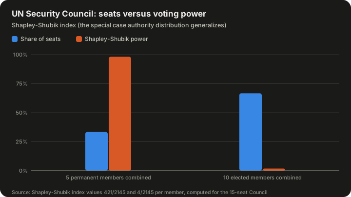
| Group | Members | Share of seats | Shapley–Shubik power (combined) | Power per member |
|---|---|---|---|---|
| Permanent members | 5 | 33.33% | 98.14% (2,105/2,145) | 421/2,145 ≈ 19.63% |
| Elected members | 10 | 66.67% | 1.86% (40/2,145) | 4/2,145 ≈ 0.19% |
Computed from the Shapley–Shubik index values given in the Wikipedia article on the index (421/2145 and 4/2145 per member).
This is exactly the kind of gap between formal membership and real power that authority distribution sets out to measure in more complicated, layered settings.
How authority distribution works
Command games
In Hu and Shapley's framework, every member of an organisation has their own command game. The game describes which groups of other members can make that person act. For a junior employee, the winning coalitions might be "my manager" or "any two of the three senior staff". For a chief executive, they might be "a majority of the board". The command game encodes both boss relations (who can give orders) and approval relations (whose agreement is needed).
Each command game is a simple game, so each has a Shapley–Shubik index. In member i's command game, the index tells us how much direct power each member holds over i.
The power transit matrix
Collect all of these indices into a square table, one row and one column per member. The entry in row i, column j, written P(i, j), is the Shapley–Shubik power of member j in member i's command game. In other words, it is the share of direct control over i that belongs to j. Because each row comes from one Shapley–Shubik index, each row adds up to 1. Wikipedia calls this table the power transit matrix; Hu's 2020 paper calls it the power transition matrix.
Mathematically, a square table of non-negative numbers whose rows each sum to 1 is a stochastic matrix, the same object used to describe Markov chains, random processes that hop from state to state with fixed probabilities.
The counterbalance equation
The authority distribution is a row of numbers π = (π1, π2, ..., πn), one per member, that satisfies
π = πP
together with the conditions that every πi is zero or positive and that they add up to 1. Hu's 2020 paper calls this the counterbalance equilibrium.
Written out for a single member i, the equation says
πi = π1·P(1, i) + π2·P(2, i) + ... + πn·P(n, i)
That is, member i's authority equals the sum, over every member j, of j's authority multiplied by i's share of direct control over j. The Wikipedia summary puts it in words: a person's power comes from their critical roles in other people's command games, and it is redistributed to the vital players in their own command game.
Two things follow from that formula, as Hu's 2020 paper spells out:
- Power from the powerful counts more. A member gains more authority from controlling an influential member than from controlling a weak one, other things being equal.
- Power flows both ways. Each member also passes authority on to whoever controls them. The more control k has over i, the more of i's authority flows to k.
The equilibrium is where inflows and outflows balance for everyone at once.
Why it is called a steady state
There is a natural story behind the equation. Start with any guess of how authority is spread, for example equal shares. Let every member pass their authority on according to the matrix: member i sends P(i, j) of their authority to j. After one round, the shares have changed. Repeat. Under fairly mild conditions, the shares settle down to a fixed pattern that no longer changes from round to round. That fixed pattern is π.
Hu's 2020 paper describes this as the accumulation of "spillover effects". Direct influence is only the first step. Member i influences z, who influences k, so i has indirect influence on k even if they never interact directly. Two-step influence is captured by the matrix P multiplied by itself (P²), three-step influence by P³, and so on. Hu proves that if P is irreducible and aperiodic (terms borrowed from Markov chain theory, roughly meaning that everyone is ultimately connected to everyone else and the chain does not cycle in a fixed rhythm), the solution of π = πP is the same as the solution of π = πP^m for any number of steps m. As m grows, all the rows of P^m converge to π, and, in Hu's words, P^m gradually smooths out all conflicts in P.
Worked example 4: two players (hypothetical)
Take a hypothetical two-player system where
| Player 1 | Player 2 | |
|---|---|---|
| Row for player 1 | 0.6 | 0.4 |
| Row for player 2 | 0.2 | 0.8 |
Player 1 holds 60% of the control over themselves, and player 2 holds 40%. Player 2 controls 80% of themselves and player 1 holds 20%.
The counterbalance equation for player 1 gives π1 = 0.6·π1 + 0.2·π2, which simplifies to 0.4·π1 = 0.2·π2, so π2 = 2·π1. With π1 + π2 = 1, the answer is π1 = 1/3 and π2 = 2/3.
The iterative story gives the same result. Start from equal shares (0.5, 0.5):
| Round | Player 1 | Player 2 |
|---|---|---|
| 0 | 0.500 | 0.500 |
| 1 | 0.400 | 0.600 |
| 2 | 0.360 | 0.640 |
| 3 | 0.344 | 0.656 |
| Limit | 0.333 | 0.667 |
Round 1, for example: player 1 receives 0.5 × 0.6 + 0.5 × 0.2 = 0.4, and player 2 receives 0.5 × 0.4 + 0.5 × 0.8 = 0.6.
Worked example 5: a small organisation (hypothetical)
The following example is invented to show the mechanics. It is in the spirit of Hu and Shapley's framework but is not taken from their papers. A small firm has a director (D), two managers (M1 and M2) and one worker (W).
- The director's command game. Major decisions by the director need ratification by a majority of the three-person leadership group {D, M1, M2}. In a three-person majority game every member is equally likely to be pivotal, so each has a Shapley–Shubik index of 1/3.
- Each manager's command game. A manager acts if either the director orders it or the manager decides alone. With two relevant players, whoever comes first in the ordering is pivotal, so the director and the manager each hold 1/2.
- The worker's command game. The worker acts only if the worker and at least one manager agree. In the six orderings of {W, M1, M2}, the worker is pivotal in four, and each manager in one, giving W 2/3, M1 1/6 and M2 1/6.
| Command game of | D | M1 | M2 | W |
|---|---|---|---|---|
| D | 1/3 | 1/3 | 1/3 | 0 |
| M1 | 1/2 | 1/2 | 0 | 0 |
| M2 | 1/2 | 0 | 1/2 | 0 |
| W | 0 | 1/6 | 1/6 | 2/3 |
Now solve π = πP. The worker's column has a non-zero entry only in the worker's own row, so πW = (2/3)·πW, which forces πW = 0. For M1: πM1 = (1/3)·πD + (1/2)·πM1 + (1/6)·πW, so with πW = 0, πM1 = (2/3)·πD. The same holds for M2. Normalising, πD + (2/3)πD + (2/3)πD = 1, so πD = 3/7.
| Member | Authority share |
|---|---|
| Director | 3/7 ≈ 42.9% |
| Manager 1 | 2/7 ≈ 28.6% |
| Manager 2 | 2/7 ≈ 28.6% |
| Worker | 0% |
The result illustrates the logic of the counterbalance equation. The worker has a great deal of say over the worker's own actions, but no one else's actions depend on the worker, so the worker holds no authority in the organisation as a whole. The managers gain authority because the director's decisions depend on them. The director gains authority because the managers' actions depend on the director. Authority is not about how free you are; it is about how much others depend on you.
The example also shows a technical subtlety. The matrix is not irreducible, because no one depends on the worker, so the worker's state is "transient" in Markov-chain language. The equilibrium still exists here, but in general the irreducibility and aperiodicity conditions matter for whether a unique answer exists and whether iteration converges.
When it reduces to the Shapley–Shubik index
For a simple legislature, there is only one decision-making body, and every member's "command game" is the same vote. In that case every row of P is identical and equal to the Shapley–Shubik index of the legislature. Solving π = πP then returns that same index. This is why Wikipedia describes the Shapley–Shubik index as a special case of authority distribution.
Authority distribution and PageRank
Readers who know how search engines rank web pages will notice a family resemblance. Google's PageRank also scores items by solving for the steady state of a stochastic matrix: a page is important if important pages link to it. Hu's 2020 paper makes the comparison directly. Compared with PageRank, he writes, authority distribution "drops the damping factor and has a stochastic matrix with a non-zero diagonal".
| Feature | Authority distribution | PageRank |
|---|---|---|
| Underlying object | Stochastic matrix of direct control or choice shares | Stochastic matrix of link-following probabilities |
| Diagonal (self-influence) | Allowed and usually non-zero, such as a college keeping its own admitted students | Usually zero; a page does not link to itself in the basic model |
| Damping factor | None | Yes; a "random jump" term mixes in a uniform probability |
| Origin | Cooperative game theory (Shapley value and power indices) | Random-surfer model of web browsing |
| Typical use | Power in organisations, ranking by revealed preference | Ranking web pages by link structure |
The two methods are close relatives in their mathematics, but they rest on different stories. PageRank's story is a random surfer clicking links. Authority distribution's story is power being passed along chains of command or choice until it balances.
Applications
The Wikipedia article on authority distribution lists several proposed applications, most of them from Hu's own papers. In each case the hard work lies in deciding what P(i, j) should mean and how to estimate it.
| Application | What P(i, j) represents | What the distribution measures |
|---|---|---|
| Organisational power | j's Shapley–Shubik power in i's command game | Each member's overall authority in the hierarchy |
| College ranking | Share of students admitted to college i who enrol at college j | Attractiveness of each college to applicants |
| Journal ranking | Share of journal i's citations that go to journal j (with P(i, i) the self-citation rate) | Each journal's long-term influence |
| Freeway planning | Estimated share of traffic on freeway i that flows onto freeway j | Relative traffic intensity, which could guide investment |
| Exchange-rate weights | Country j's share of the consumption of country i's production | Weights in an n-country trading system |
Wikipedia also notes that a similar question arises in Internet and intranet design. In his 2020 paper Hu also suggests sports team rankings and voting as further possible uses.
Case study: ranking twelve US colleges
The most fully worked-out application is Hu's 2020 college-ranking paper. It is worth looking at in detail because it shows both the appeal of the method and its practical difficulties.
The motivation
Hu starts from a familiar complaint about commercial college rankings: they mostly rely on a preset weighting of a handful of criteria, such as acceptance rates, test scores, alumni giving and class sizes. The choice of criteria and weights is subjective, and small changes in weights can shuffle the results. To illustrate how much rankings disagree, the paper's Table 1 shows that UCLA's position across a dozen published rankings (accessed in March 2019) ranged from 5th to 31st, so its lowest rank was six times its highest.
His alternative is to let students' actual choices do the weighting. When a student is admitted to several colleges and picks one, that choice reveals a preference that already takes into account everything the student cares about, from tuition to distance from home to the feel of the campus. Each college is treated as a player, and the students who are admitted to it and then choose where to go form a "foot voting" game.
Building the matrix
In this setting, P(i, j) is the probability that a student admitted to college i ends up enrolling at college j. The diagonal entry P(i, i) is simply the college's enrolment yield: the share of admitted students who enrol. Official admissions data give this with good precision. For example, the paper's Table 2 reports that UCLA admitted 15,988 of 113,779 applicants for fall 2018 and 6,240 of those admitted enrolled, a yield of 39.03%.
The off-diagonal entries are harder. Hu estimates them from survey data of student preferences posted on sites such as Parchment and Niche. The paper's example: among students admitted to both Harvard and Stanford who chose one of the two, 56% chose Harvard and 44% chose Stanford, with a 95% confidence interval for the 56% figure of 51.2% to 60.7%, as listed on Parchment.
Why simple head-to-head comparisons are not enough
The paper points out several problems with the raw head-to-head data that the authority distribution is meant to fix:
- Preferences are not transitive. Using bilateral comparisons alone, there is a cycle in the data: Michigan is preferred to Virginia, Virginia to UCLA, and UCLA to Michigan.
- Odds do not multiply. UCLA beats Michigan 43 to 57 and UCLA beats Berkeley 47 to 53 in head-to-head choices, but these do not imply the Berkeley-versus-Michigan figure; in the data Michigan actually trails Berkeley 39 to 61.
- Benchmarks disagree. Ordering colleges by how they fare against Harvard gives a different order from ordering them by how they fare against Berkeley.
- Geography matters. Berkeley has its lowest odds against Stanford, its nearest neighbour on the list; UCLA has its lowest odds against Caltech, also its nearest.
The authority distribution resolves these conflicts by weighting each comparison by the authority of the colleges involved and letting the spillovers run until they settle.
The results
Hu applied the method to a "mini sample" of twelve colleges: seven private and five public institutions that mainstream rankings often place near the top. He reports scores with 95% confidence bands, plus the mean and median of 20,000 simulated sets of scores.
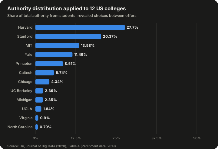
| Rank | College | Score (share of total authority) | 95% interval for score |
|---|---|---|---|
| 1 | Harvard | 0.2770 | 0.2757–0.2784 |
| 2 | Stanford | 0.2037 | 0.2024–0.2049 |
| 3 | MIT | 0.1358 | 0.1347–0.1368 |
| 4 | Yale | 0.1149 | 0.1142–0.1155 |
| 5 | Princeton | 0.0851 | 0.0844–0.0858 |
| 6 | Caltech | 0.0574 | 0.0567–0.0583 |
| 7 | Chicago | 0.0434 | 0.0430–0.0439 |
| 8 | UC Berkeley | 0.0239 | 0.0236–0.0243 |
| 9 | Michigan | 0.0235 | 0.0230–0.0239 |
| 10 | UCLA | 0.0184 | 0.0181–0.0188 |
| 11 | Virginia | 0.0090 | 0.0087–0.0094 |
| 12 | North Carolina | 0.0079 | 0.0075–0.0084 |
Source: Hu, Journal of Big Data (2020), Table 4, using Parchment preference data accessed 1 November 2019.
Several features stand out:
- Concentration at the top. Harvard and Stanford together hold 48.07% of the total authority, "nearly half" in Hu's words. Harvard's score is about 36% higher than Stanford's (0.2770 / 0.2037 ≈ 1.36; the paper rounds this to 40%), even though their head-to-head odds were a relatively close 56 to 44. The paper attributes this to the spillover's amplification effect: Harvard's advantages over every other college compound through the network.
- Private ahead of public. All seven private colleges in the sample score above all five public ones.
- Ties that need more data. Berkeley and Michigan are separated by only 0.0004, and their confidence intervals overlap; their rank intervals are both "8 to 9". Hu suggests that adding more colleges to the sample would help separate them.
What the matrix reveals
The estimated matrix also shows who influences whom. Reading down Harvard's column, Hu notes that Harvard pulls authority from Yale, Princeton, Caltech and Michigan, in decreasing order. Reading along UCLA's row, the four colleges with the most direct influence on UCLA are Berkeley, Caltech, MIT and Stanford. The influence on North Carolina is the most evenly spread, which Hu suggests may reflect its distance from the other institutions in the sample.
Strategies to improve a score
Because the score is an explicit function of the matrix, it is possible to ask how a college could raise it. Hu derives formulas for how a college's score responds to a small change in its own yield, and he reports the percentage response of each college's score to a 1% increase in its yield. The responses range widely, from 0.621 for Caltech to 2.79 for Harvard. That range, he argues, is itself evidence that a standard regression model with a single coefficient on enrolment rates would be "highly artificial".
He gives a worked case. For Michigan to catch up with Berkeley, its score would need to rise by 0.0239 / 0.0235 − 1 ≈ 1.7%. Since Michigan's score responds to its yield with an elasticity of 0.668, that would take roughly 1.7 / 0.668 ≈ 2.55% more yield, other things unchanged.
Hu warns against treating yield alone as a ranking: a college could inflate its yield simply by admitting less competitive applicants. The authority distribution guards against this because it counts where the students who turn a college down go instead, and gains more weight from winning students away from strong competitors.
Strategyproofness and partnerships
Two further results in the paper deal with incentives:
- Students have no reason to hide their choices. Hu proves (his Theorem 5) that when a student who chose college i over college j reports that choice, i's score cannot fall. Both the college and the student are better off if the choice is revealed, so there is no incentive for students to hide it. He calls this strategyproofness.
- Colleges can be partners as well as rivals. Because a college's authority partly flows from the authority of the colleges it beats, a college can sometimes gain when a rival gains. The paper identifies pairs where this works in both directions, such as Harvard and Yale, MIT and Caltech, and Michigan and Chicago, as well as three-way groups such as Michigan, Virginia and North Carolina.
Stated limits
Hu is explicit that he is illustrating a method, not publishing a rival league table. Ranking all of the roughly 3,000 US colleges would be costly in data and computation, and any truncated list distorts the results to some degree. The online preference surveys are self-reported and may not represent all students. The paper's view is that a ranking of moderate size should ideally be updated in real time as new choice data arrive.
Key properties
Pulling the strands together, authority distribution has these main properties, as set out in the Wikipedia summary and Hu's 2020 paper:
| Property | What it means |
|---|---|
| Normalised | Shares are non-negative and sum to 1, so they can be read as fractions of total authority |
| Generalises Shapley–Shubik | For a single legislature it gives exactly the Shapley–Shubik index |
| Recursive | Authority from powerful players counts more than authority from weak ones |
| Two-way flow | Each player both receives authority from those they control and passes it to those who control them |
| Captures indirect influence | Multi-step chains of influence are included through powers of the matrix |
| Steady state | Under irreducibility and aperiodicity the solution is unique and iteration converges to it |
| Endogenous weights | The weights given to each comparison come from the system itself, not from an outside analyst |
| Incentive properties (ranking case) | Revealing a true choice cannot hurt the chosen college; yield can raise a college's own score but not others' |
Strengths
- It makes hidden power visible. Like the Shapley–Shubik index, it can show that formal seats or titles misstate real influence.
- It handles hierarchy and indirect influence. Single-body power indices cannot easily describe chains of command; authority distribution was designed for them.
- It removes arbitrary weights. In ranking applications, it replaces a panel's chosen weights with weights that come from the network itself.
- It has a clear mathematical foundation. It rests on the Shapley value's axioms and on the well-understood theory of stochastic matrices, and it can be computed with standard linear-algebra methods.
- It supports "what if" analysis. Because the score is a known function of the matrix, sensitivities and partnerships can be calculated, as in Hu's college example.
Limitations and criticisms
Garbage in, garbage out
The method is only as good as the matrix. In organisations, someone has to decide what each member's command game looks like: who really can order whom, whose approval is truly required, and what counts as a winning coalition. Real organisations run on informal relationships, expertise and information as much as on formal approval rights, and a model built from an organisation chart may miss most of that. In the college case, the off-diagonal entries come from voluntary online surveys, which Hu himself treats as less precise than official yield figures.
Inherited assumptions of the Shapley–Shubik index
Because each row of the matrix is a Shapley–Shubik index, the method inherits that index's assumptions. The Wikipedia article on the index lists the main ones: all orderings are treated as equally likely, and members are assumed to vote independently of party, preferences or agenda control. Real decision-making bodies often break these assumptions through party discipline, procedure, logrolling or control of the agenda, so actual influence after the fact can differ from the a priori power the index measures. The index remains useful as a benchmark, but it is a model of potential, not a forecast of behaviour.
Computation
Exact Shapley–Shubik indices require looking at n! orderings, and computing Shapley-value-based indices for general games is known to be computationally hard (#P-complete). Authority distribution then requires building and solving a matrix equation on top of those indices. For small organisations this is easy; for large ones, approximation methods or special structure are needed.
Existence and uniqueness
The neat convergence story depends on the matrix being irreducible and aperiodic. If parts of the organisation do not influence each other at all, or if influence runs in strict cycles, the equilibrium may not be unique, and some members may end up with zero authority by construction, as the worker did in the hypothetical example above. Analysts have to check these conditions rather than assume them.
Limited independent literature
The Wikipedia article on authority distribution carries a warning that it relies excessively on primary sources. Most published applications come from Hu himself. Hu's 2020 paper notes that the distribution has been used in work on social networks, corporate networks and control (citing, for example, Crama and Leruth in 2007 and Grabisch and Rusinowska in 2010), but the concept is far less widely used than the Shapley value or the Shapley–Shubik and Banzhaf indices. Readers should treat claims about its practical success with appropriate caution until more independent studies exist.
Common misconceptions
"Authority distribution measures how much freedom a person has." No. It measures how much others depend on a person. In the small-firm example above, the worker had most of the control over the worker's own actions but zero authority overall.
"More votes always means more power." The Shapley–Shubik examples show otherwise. A member with twice the weight of another can have exactly the same power, and a 50% shareholder can hold two-thirds of the power.
"It is just PageRank under another name." The mathematics is closely related, but authority distribution has no damping factor, keeps self-influence on the diagonal, and comes from cooperative game theory rather than a random-surfer model. In organisational settings, its matrix is built from power indices of command games, which PageRank has no counterpart for.
"Hu's college scores are a league table of the best colleges." Hu describes the twelve-college ranking as an illustration of the method, based on a truncated list and on survey data, not as a competitor to commercial rankings. The scores measure relative attractiveness to admitted students within that sample, nothing more.
"The Shapley–Shubik index is a different thing altogether." It is the special case. For a single voting body with no hierarchy, the two give the same numbers.
Frequently asked questions
Who invented authority distribution?
Xingwei Hu and Lloyd Shapley, in two papers published in Games and Economic Behavior, volume 45, in 2003.
What does the equation π = πP mean in plain language?
It says that each member's authority equals the sum of the authority of every member they help control, weighted by how much control they have. Everyone's authority is defined in terms of everyone else's, and the equation picks out the one consistent set of values where all those definitions agree.
How is it different from a voting power index?
A voting power index, such as the Shapley–Shubik or Banzhaf index, measures power within one voting body. Authority distribution links many such "games" together, one for each member of an organisation, and finds the overall balance of power across all of them.
Do I need to know game theory to use it?
To apply it to an organisation, you need to define each member's command game, which requires knowing what a simple game and a winning coalition are. For ranking applications, the matrix can be built directly from data such as choice shares or citation shares, and the calculation is ordinary linear algebra.
How is it computed?
Either by solving the linear system π = πP with the condition that the shares sum to 1, or by repeatedly multiplying a starting vector by P until it stops changing. Hu's 2020 paper uses an iterative algorithm and simulation to estimate confidence intervals.
Has it been used outside academic papers?
The published applications are mostly illustrative, such as Hu's twelve-college ranking. There is no evidence in the sources reviewed here of authority distribution being widely used in official rankings, corporate governance or policy.
What are the online tools for power indices?
The Wikipedia article links to several power-index calculators, including tools hosted by Tomomi Matsui and at the University of Kiel, and a collection of algorithms for voting power analysis from the University of Warwick. These compute standard indices such as Shapley–Shubik and Banzhaf rather than authority distributions directly.
Summary
Authority distribution is a game-theoretic measure of power in networks where members influence one another through chains of command, approval or choice. Proposed by Xingwei Hu and Lloyd Shapley in 2003, it builds a matrix of direct influence from Shapley–Shubik power indices and then solves the counterbalance equation π = πP to find the steady-state share of authority held by each member. It reduces to the Shapley–Shubik index for a simple legislature, shares much of its mathematics with PageRank, and has been applied most fully to ranking colleges from the choices of admitted students, where it put Harvard and Stanford at nearly half of the total authority among twelve elite institutions. Its strengths are its clear foundations and its ability to capture indirect influence without arbitrary weights. Its weaknesses are its dependence on a good matrix, the strong assumptions inherited from power indices, computational cost for large systems, and a still-thin body of independent research.
Sources
- Authority distribution — Wikipedia
- Shapley–Shubik power index — Wikipedia
- Hu, X. (2020). Sorting big data by revealed preference with application to college ranking. Journal of Big Data 7 (arXiv:2003.12198)
- Hu, X. and Shapley, L. S. (2003). On authority distributions in organizations: equilibrium. Games and Economic Behavior 45(1), 132–152 (IDEAS/RePEc record)
- Hu, X. and Shapley, L. S. (2003). On authority distributions in organizations: controls. Games and Economic Behavior 45(1), 153–170 (IDEAS/RePEc record)
- Hu, X. (2006). An asymmetric Shapley–Shubik power index. International Journal of Game Theory 34(2), 229–240
- Shapley, L. S. and Shubik, M. (1954). A method for evaluating the distribution of power in a committee system. American Political Science Review 48(3), 787–792