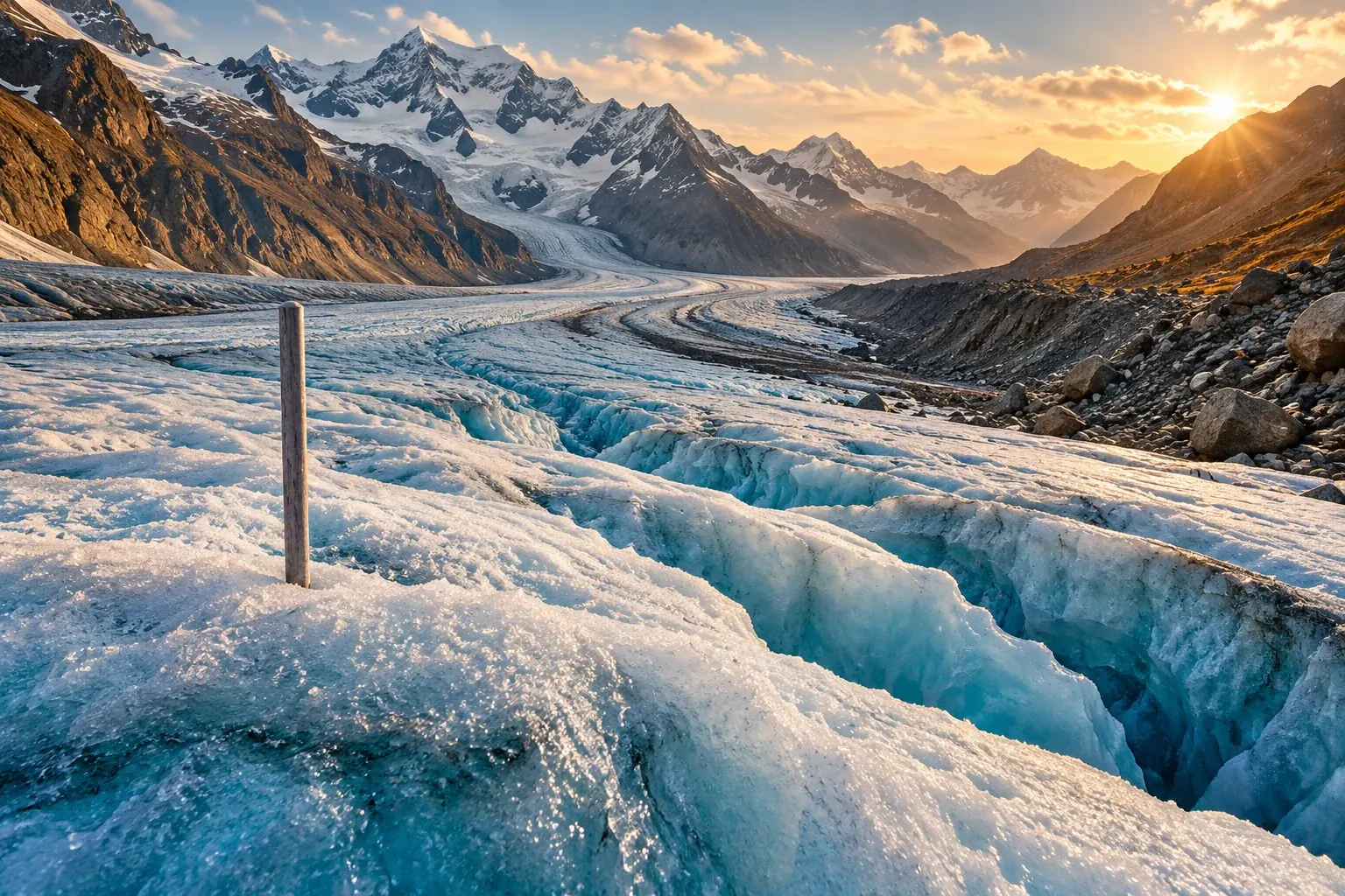
Field stakes, elevation maps, and global comparisons reveal different parts of the ice-loss story. Understanding their units makes the evidence clearer.
A glacier can become thinner, shorter, smaller in area, or lighter. Those changes are related, but they are not interchangeable measurements. A photograph of a retreating terminus tells a visible story about the position of an edge. A mass-balance estimate asks a different question: how much material the glacier gained or lost over a stated interval. Turning observations into that estimate requires decisions about space, time, density, and uncertainty that rarely fit inside a climate headline.
The latest annual result used here is a study published on April 7, 2026, reporting a global glacier mass loss of 408 ± 132 gigatonnes during the hydrological year 2025, equivalent to 1.1 ± 0.4 millimeters of global sea-level rise. The USGS publication record provides that research summary. It is a dated assessment of the specified year, not a measurement of conditions on November 1, 2026, and its sea-level equivalent should not be read as a prediction for the waterline at an individual beach. Primary author publication record.
A longer perspective comes from the GlaMBIE collaboration's February 2025 intercomparison. It combined several observation approaches and estimated average annual glacier mass loss of 273 ± 16 gigatonnes over 2000–2023, with a thirty-six ± ten percent increase between the first and second halves of that interval. The assessment concerns glaciers distinct from the Greenland and Antarctic ice sheets. Its authors also discussed correlated errors and remaining limitations in combining methods, rather than claiming that agreement had removed every uncertainty. Original intercomparison.
The difference between those two headline rates is not, on its own, a contradiction. One describes a particular hydrological year; the other describes an average across a long interval. Their periods and methods need to be understood before the numbers are compared. This article follows the measurement chain from a point on the ice to a regional or global estimate, using primary research and original worked examples to show what the numbers can support and where careless comparisons go wrong.
Begin with the boundary of the question
Before weighing anything, define what belongs inside the accounting boundary. For a glacier, the boundary can be geographical, temporal, and conceptual. Does the estimate concern the entire glacier or a monitored part? Does it describe a season, a hydrological year, or the interval between two surveys? Does it refer to surface mass balance or a broader total that includes additional processes? The label mass balance needs that context to become a clear scientific statement.
A simple hypothetical accounting example helps. Imagine a defined body that receives twelve units of material and loses fifteen units over a year. Its net change is a loss of three units. The total amount that left is fifteen, not three. Confusing gross loss with net change would misdescribe the account even though both numbers concern material leaving or being depleted. This example illustrates bookkeeping logic; it is not a model of a real glacier or a complete inventory of glaciological processes.
The distinction matters when melt is used casually as a synonym for all mass loss. A study may estimate a net change without observing every individual pathway by which material entered or left. A reader should use the quantity the authors actually report rather than replacing it with a more familiar word that changes the meaning. A careful headline can remain accessible while preserving that distinction.
A boundary also determines which observations belong in the comparison. If one survey includes an area that another excludes, the difference can reflect both a physical change and a change in the object being measured. This is a familiar problem in maps: redrawing a district can alter its population total without anyone moving. For glacier analysis, the relevant geometry and reference area must be identified so that the reported change describes the intended object.
The time boundary deserves equal attention. A measurement taken near the end of one season cannot simply be compared with a measurement taken at a very different seasonal stage without considering what happened between them. A date is not a minor annotation to an elevation map. It helps define the quantity being inferred from the difference between maps.
These choices do not make the result arbitrary. They make it interpretable. Scientific accounting becomes stronger when the boundary is explicit and the methods explain how observations are brought into it. A number without that description may be easy to repeat, but it is harder to compare, reproduce, or use for a decision.
A stake observes a place, not an entire mountain
Field monitoring provides detailed information at selected locations. Its strength is the connection between an observation and the material at that point. Its challenge is how to represent a much larger, varied surface using a finite set of observations. The movement from point measurements to a glacier-wide estimate is therefore part of the analysis, not an automatic consequence of having visited the glacier.
The USGS's March 2026 methods account describes spring measurements of snow depth and density and later measurements of seasonal ablation, distributed across glacier elevation ranges. Those observations are extrapolated across the glacier, while remotely sensed geometry provides an additional check on longer-term change. This is a first-party description of the monitoring program's methods, not a claim that every glacier worldwide is observed with the same field network. USGS methods record.
Imagine a hypothetical glacier divided into three elevation bands with different areas. If a measurement from each band is simply averaged, a small band receives the same weight as a large one. That may not answer the question of average change over the entire surface. An area-weighted calculation would account for how much of the glacier each band represents. The example does not prescribe an actual field method; it demonstrates why the spatial weights matter.
Suppose the three invented bands occupy one, two, and seven equal area units, and their measured changes are minus one, minus two, and plus one mass-per-area units. The unweighted mean is minus two thirds. The area-weighted mean is positive two tenths, because the largest band contributes most of the total area. Both calculations use the same three observations, but only one incorporates the stated geometry. The contrast is deliberately simplified to make the role of weighting visible.
Real analysis must additionally consider whether a point represents its assigned area, how the surface changes, and how measurement errors propagate. More observations can help, but they do not eliminate the need to think about representativeness. A dense cluster in an accessible location may provide excellent local information while leaving another part of the glacier poorly constrained.
This is why field programs and broad-area observations are complementary. The question is not which method deserves to replace the other in a dramatic technological contest. It is which aspects of the change each method observes well, and how their different strengths can be combined without concealing their limitations. A long field record can retain value even as remote measurements become more extensive.
Elevation change is a geometric observation
A digital elevation model represents the height of a surface over an area. Comparing such representations from different times can reveal a change in surface geometry. That observation is powerful because it can extend beyond the places people can readily visit. But a height difference is not yet a mass difference. The conversion requires the area over which the change occurs and assumptions or information about the material involved.
Hugonnet and colleagues' 2021 global study used satellite image archives to reconstruct glacier surface-elevation changes over 2000–2019 and validate estimates against independent measurements. The published result reported average mass loss of 267 ± 16 gigatonnes per year. The author-accepted manuscript was accessible for this article; the publisher page was not. The study's contribution here is a concrete example of turning extensive geometric observations into a global mass-change estimate with explicit validation and uncertainty. Original accepted manuscript.
A hypothetical tabletop model makes the geometric step easy to see. If a flat one-square-meter patch becomes ten centimeters lower everywhere, its volume has decreased by one tenth of a cubic meter. If the patch were twice as large with the same uniform height change, the volume change would double. The calculation is simple because the surface is deliberately idealized. Actual glacier geometry requires integrating variation over a mapped area rather than assuming the whole surface changes uniformly.
A map difference also depends on alignment. If two representations of unchanged terrain are offset, subtracting them can produce apparent changes. Analysts therefore need ways to assess the relationship between datasets and identify biases. The general principle is familiar from comparing two photographs: a shifted viewpoint can create apparent movement that does not correspond to the feature's actual displacement. Quantitative surface comparison requires a more rigorous treatment than visual matching.
Data gaps introduce another issue. A complete-looking map may include areas estimated from surrounding information rather than directly observed at every date. That can be scientifically appropriate, but the distinction should remain documented. A reader should not assume that every colored pixel represents an independent measurement with identical certainty. The methods determine how observations, interpolation, and uncertainty relate.
This also explains why a striking local patch should not be used casually to describe the whole glacier. The most dramatic change in a map can be real while differing from the area-wide average. Selecting the largest visible thinning value may help illustrate spatial variation; presenting it as the typical change would alter the claim. A useful graphic shows both the pattern and the quantity that the headline summarizes.
Density is where the geometry becomes mass
The relation between volume and mass depends on density. A cubic meter of loosely packed snow and a cubic meter of compact ice do not contain the same mass. A change in surface height can also involve changes in the internal structure of snow and firn. These distinctions explain why a single geometric observation cannot always be converted into mass with one universally reliable factor.
Huss's 2013 study investigated density assumptions using a firn-compaction model and long-term glacier records. It found that an effective conversion factor around 850 ± 60 kilograms per cubic meter was appropriate across a broad range of conditions, while short intervals and certain changing conditions could produce much more variable effective factors. This is a finding about converting geodetic volume change, not a claim that all glacier material has that density. Original study.
The word effective matters. A conversion factor summarizes how a measured volume change relates to mass change over the defined interval. It need not equal the density of a single homogeneous block imagined in a classroom. If the geometry changes partly because material compacts, the relation between the surface displacement and net mass change can differ from the relation for simple removal of a uniform block.
An original hypothetical comparison shows why. Take two containers with the same initial surface height. In one, material is removed. In the other, the existing material becomes more tightly packed without any leaving. Both surfaces can become lower, but their mass changes differ. A glacier is far more complex than these containers, yet the example isolates the logical reason that surface lowering and loss of mass cannot be assumed to be identical operations.
The uncertainty in a conversion should follow the calculation. If the geometric change is known precisely but the effective density is uncertain, the final mass estimate still has uncertainty. Improving one input does not automatically remove the limitation of another. This is a general lesson in measurement chains: the precision of the most visible instrument is not necessarily the precision of the final inferred quantity.
Public reporting often emphasizes the satellite because it is an appealing technological protagonist. The less visible conversion assumptions may be just as important to understanding the result. An informative article gives both their proper roles. It can explain that the observation is sophisticated and the estimate useful while still identifying the assumptions needed to move from one to the other.
Why a long record may be revised
A revised historical estimate can look suspicious to a reader who imagines data as a set of immutable facts written down once. In practice, observations and derived estimates are different layers. An original measurement can remain unchanged while a better calibration, a corrected geometry, or a more consistent analytical method changes the estimate derived from it. The important question is whether the revision is documented and justified.
O'Neel and colleagues' 2019 reanalysis of five USGS Benchmark Glaciers applied consistent extrapolation and calibration approaches to long records. It found cumulative mass loss across the studied glaciers and showed the value of geodetic calibration alongside direct observations. The paper is a specific example of reanalysis improving comparability and uncertainty characterization, rather than a reason to assume every future revision will move in the same direction. Original reanalysis.
An invented laboratory analogy is useful. Suppose a researcher measures a series of objects with an instrument and later discovers a documented calibration offset. Correcting the derived results does not require pretending the original readings were never made. A good archive retains the readings, the earlier calculation, the correction, and the reason for it. The revised estimate becomes more trustworthy because its history is visible.
Long environmental records can face more complicated versions of that problem. Methods change, observation coverage changes, and the object being measured changes. A consistent reanalysis can help distinguish those effects from the physical signal of interest. The process should not be described as automatically improving a result merely because it is newer; it should explain which limitation the revision addresses and how the evidence supports the change.
This has practical consequences for users of published data. A graph downloaded several years ago may not match the latest version exactly. Before declaring a contradiction, check whether the versions use the same method, period, and input set. Before replacing the old graph, preserve its citation and identify the revision. Version-aware reporting avoids both the illusion that numbers never change and the equally misleading suggestion that any change makes them meaningless.
It also helps separate uncertainty from disagreement. Two estimates can differ within their stated uncertainty ranges, or differ because they define the quantity differently. A real unresolved discrepancy may remain after those issues are considered. That discrepancy is worth studying. The first step is to make the comparison fair enough that the remaining difference means what the reader thinks it means.
A year is not always January through December
The term annual can conceal a calendar choice. A hydrological year is selected to organize the relevant seasonal cycle, and its dates can differ by region or application. A calendar-year estimate and a hydrological-year estimate may include different months. Comparing them as though they refer to exactly the same interval can create an apparent disagreement that partly reflects timing.
A hypothetical example makes the issue concrete. Imagine an unusually strong loss period near the boundary between two accounting years. A series ending just before that period assigns the loss to the next year; a series ending afterward includes it in the current one. The multi-year totals could be similar while individual annual values differ. The dates need to accompany the annual label if the comparison is to be interpreted correctly.
Seasonal observations also require a defined convention. A field visit records conditions on the date of the visit, while an annual estimate may refer to a standard endpoint that falls earlier or later. The methods should explain how the interval between the observation and the endpoint is handled. An estimate can include modeled adjustments without becoming purely hypothetical, provided those adjustments and their uncertainty are made clear.
This is particularly relevant to the most recent year of a record. Some inputs may still be preliminary, or later observations may refine the estimate. A public dashboard should distinguish preliminary status from final status instead of displaying both with identical implied certainty. A revision policy can tell users when to expect updates and how to cite the version they used.
The choice of interval also affects trends. A short run of annual values can be strongly influenced by where the period starts and ends. A longer series provides a different perspective, but it still needs the definition of its years and the method used to estimate the trend. Reporting a trend without those details can make a precise-looking rate harder to evaluate than a plainly described set of observations.
For readers, the useful habit is to ask for the interval before comparing the magnitude. A result for a single hydrological year, a twenty-year mean, and an acceleration per decade are different quantities. They can all illuminate glacier change. They should not be placed on one list as though each were a competing answer to the same question.
Combining annual detail with broad coverage
Some observations provide relatively detailed timing at a limited number of glaciers. Others provide broad spatial coverage over longer intervals. Combining these strengths can produce a more informative record, but the combination is an analytical procedure that needs validation. It should not be described as though every glacier was directly measured every year by the same method.
Dussaillant and colleagues' May 2025 data paper developed annual glacier mass-change estimates through temporal downscaling of geodetic observations with in situ records. It described how annual anomalies from field observations were interpolated and calibrated to longer-term glacier-wide trends, with cross-validation and uncertainty analysis. The resulting annual series are observation-based estimates assembled through that method, not a global network of annual direct field measurements at every glacier. Original data study.
The distinction between input and output resolution is central. A product can provide one value per year for each mapped glacier even though its inputs have different temporal and spatial resolutions. The output is useful if the method supports that inference and the uncertainty is appropriate. The presence of a value in every cell does not mean the same amount of independent information exists in every cell.
An original hypothetical weather analogy illustrates the logic without asserting equivalence between the sciences. Suppose long-term totals are known for many locations, while yearly fluctuations are observed at fewer sites. A model may use the observed fluctuations to help distribute the totals through time. Its annual estimates then depend on how well those fluctuations represent the unobserved locations. Validation should test that relationship rather than merely confirming that the totals add up.
Cross-validation can withhold some observations and examine how well the method estimates them. The design of that exercise matters. Withholding isolated points may be easier than withholding a whole region or a block of time if nearby information is strongly related. A convincing evaluation should consider the kinds of gaps the final product must bridge. The article does not reproduce a particular study's full validation protocol; it explains why the choice of test affects what a successful result demonstrates.
Users of the combined product should retain its method citation when presenting a derived chart. Calling it satellite data alone could erase the contribution of field observations and the analytical steps connecting them. Calling it measured everywhere could overstate direct coverage. A precise description can be both short and informative: an observation-based estimate combining specified sources over a stated period.
The average depends on what receives weight
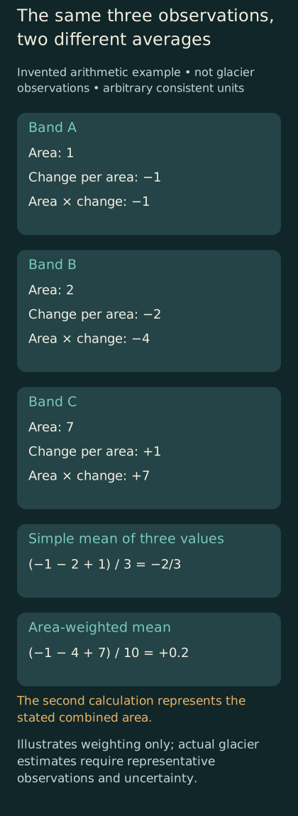
Original hypothetical weighting example. Arbitrary consistent units show why an average across three observations differs from an area-weighted mean; these are not measured glacier data.
A global average can be constructed in several ways. An average across glaciers by number gives each glacier equal weight. An area-weighted average gives larger surfaces more influence. A total mass change sums contributions rather than averaging them. These quantities answer different questions, and their numerical relationships should not be assumed from the word global alone.
Consider two invented glaciers. One has an area of one unit and loses two mass units; the other has an area of nine units and loses nine mass units. Their mass losses per unit area are two and one. The simple mean of those two intensities is one and a half. The total loss divided by total area is eleven tenths. Both are valid calculations under their definitions, but the second represents the area-wide mean for the combined surface.
The difference becomes important when a dataset contains many small glaciers and fewer large ones. A statistic describing the typical glacier by count can differ from a statistic describing the typical square kilometer of glacierized area. Neither should be substituted for the other without explanation. A headline about percentage loss can introduce yet another denominator: the amount initially present.
A region with a small initial ice stock can lose a large percentage of that stock while contributing less total mass loss than a much larger region with a smaller percentage decline. This arithmetic does not diminish the local significance of a large relative loss. It shows why rankings by absolute loss and percentage loss can legitimately differ. A chart should label which ranking it presents.
The same issue arises when comparing rates expressed in water-equivalent depth and gigatonnes. The first describes mass change relative to area; the second describes total mass change. A glacier or region can have a strong area-normalized loss without dominating the global total. Readers should resist interpreting a larger number as a larger effect until the units and denominator are aligned.
A useful editorial practice is to keep the question attached to the metric. Are we asking where the most mass was lost, where the loss was most intense per unit area, or where the largest share of the initial stock disappeared? Each question can matter for a different reason. Presenting them separately is clearer than forcing them into a single league table of which glacier is doing worst.
Uncertainty has a structure
The plus-or-minus term beside an estimate is easy to treat as a decorative sign of scientific caution. In fact, its interpretation depends on how the authors calculated it and what level of confidence or variability it represents. Different studies may report different conventions. A comparison should check those conventions before treating the sizes of the error bars as directly comparable.
Uncertainty can arise from measurements, spatial extrapolation, density conversion, temporal adjustment, and other analytical steps. Some errors may be independent; others may be shared across observations or methods. That structure affects how uncertainty behaves when results are combined. Adding more estimates does not guarantee that shared errors disappear.
A simple hypothetical example makes the point. If several thermometers all share the same calibration offset, averaging them can reduce some random variation while retaining the common offset. The average may look stable without being free of bias. This is a general statistical illustration, not a claim that glacier instruments behave like identical thermometers or that a named assessment has ignored shared errors.
The distinction between precision and accuracy follows naturally. A result can be repeatable under the same method while still affected by a systematic issue. Independent checks are valuable when their limitations differ enough to challenge that issue. Merely producing several outputs from the same input source does not create the same kind of independence as a genuinely different observation approach.
Uncertainty also does not mean that every conclusion is equally plausible. An estimate can have a substantial interval while still supporting a clear direction of change. A reader should examine the interval and the question being asked rather than treating the presence of uncertainty as a reason to discard the result. Conversely, a narrow interval for one quantity does not automatically justify a confident claim about a different consequence.
The most helpful public explanation states which conclusion is robust and which remains sensitive to assumptions. It avoids both false certainty and a fog of indiscriminate caveats. The goal is to help readers understand how much weight the evidence can bear, not to make every sentence sound equally tentative.
From mass change to a water problem
A global mass-loss estimate has relevance to sea level and freshwater, but it does not answer every local water question. The amount of ice lost across the world is not a direct forecast of discharge in a particular basin on a particular date. A basin's water problem depends on timing, storage, other sources of water, and demand, among additional site-specific factors. Moving from global observation to local consequence requires another analytical step.
The difference can be illustrated with an invented storage account. A reservoir may release more water temporarily while its stored volume declines. Increased short-term release and reduced remaining storage can occur together. This analogy explains why a flow observed during depletion should not automatically be read as evidence of a secure long-term supply. It does not predict the timing or magnitude of runoff for any real glacier-fed basin.
A local assessment would need to define the relevant season and use. Water available during one period may not resolve shortages in another. A total annual volume can hide a timing mismatch. The appropriate question for a community could concern dry-season availability, a particular ecosystem, infrastructure operations, or another objective. The glacier mass record informs that question but does not silently choose it.
Sea-level equivalent requires similar care. It is a way to express mass change in a common global unit under the study's accounting assumptions. It is not an instruction to add the same vertical increment to every local coastline without considering the processes that affect local sea level. The equivalent helps compare contributions; local planning requires a more specific assessment.
These distinctions make the global evidence more useful rather than less important. A broad estimate establishes the scale and trajectory of change. A regional or local study translates the relevant part of that change into a particular problem. Confusing those levels can lead either to exaggerated precision or to the mistaken claim that global evidence has no practical relevance because it does not answer a household's exact question.
A strong report therefore identifies the bridge it has crossed and the one it has not. It may describe measured or estimated mass change, a modeled hydrological consequence, or a planning scenario. Each can be valuable. The reader should be able to tell which kind of statement is being made.
Keeping the record reproducible
A chart is easier to trust when another person can identify the exact data and method behind it. That requires more than a link to a homepage that changes over time. It requires a version, a date, the relevant selection of records, and a description of any calculations used to create the displayed values. Reproducibility begins with preserving the identity of the evidence.
The World Glacier Monitoring Service's data-exploration page, accessed on November 1, 2026, distinguishes versioned database snapshots with digital object identifiers from its live database view. It recommends the versioned route for reproducible research. The database records several forms of glacier state and change, with source metadata. This is a primary description of the data infrastructure, not a new estimate of global mass loss. WGMS data record.
For an editor, a minimal reproducibility note could state the downloaded version, the geographical selection, the time interval, the variable and units, and the calculation used for the chart. If the chart excludes records with missing values, that choice should be documented. If it combines datasets, the combination should be explained. These details can fit in a methods note without overwhelming the main article.
The original data should be preserved separately from derived files. A spreadsheet that overwrites input values with rounded display values makes later checking harder. A better workflow retains the source values and creates a separate presentation layer. The same applies to unit conversions and sign conventions: store the transformation so that another reader can reconstruct it.
A correction should update the public result while preserving the history of what changed. If a caption confused volume and mass, the correction should say so. If a revised dataset changes a value, the new version should be identified. Transparent maintenance supports confidence more effectively than silently replacing an old chart and hoping nobody notices the difference.
This is especially important for long-lived articles. A piece prepared in November 2026 can remain useful as an explanation of methods, but its latest annual result will eventually become historical. Clear dates allow that transition without making the article misleading. The method discussion and the dated evidence can coexist, provided the article does not imply that its numbers update automatically.
A quick audit of a glacier graphic
A glacier chart should let its visual form follow the quantity. A line showing cumulative change needs an identified starting reference. A bar showing annual change needs a defined year. A map showing mass change per unit area needs units that differ clearly from a map of total mass change. These choices affect the message before a reader has examined a single value.
Sign conventions deserve particular care. One graphic may show losses as negative mass change; another may show the magnitude of loss as a positive number. Both can be clear when labeled. Combining them on the same axis without explanation can reverse the apparent direction of change. A caption should state whether the plotted quantity is signed net change or a positive loss magnitude.
Color should support that distinction rather than carry it alone. A reader who cannot distinguish two hues should still be able to identify what the values mean through labels, positions, or patterns. Decorative gradients should not imply measurements between observations unless the interpolation is part of the stated method. A smooth curve drawn through sparse annual values can suggest a temporal detail the observations do not provide.
The caption should also identify what has not been plotted. A glacier-only chart should not be read as the complete contribution of all land ice. A selected regional series should not be mistaken for the global record. A hypothetical calculation should say that it is hypothetical directly beside the figure, rather than relying on a distant methods paragraph. These small choices preserve the boundary between a helpful illustration and a misleading claim.
Finally, the graphic should remain understandable when separated from the article. Shared images often lose their surrounding text. Including the period, units, source identity, and conceptual or measured status within the image or its attached caption reduces the chance that a useful chart becomes misinformation through incomplete redistribution.
A glacier record is more than a shrinking outline
The visible retreat of ice can be compelling, but the mass-balance record adds a different kind of knowledge. It connects observations to a defined quantity, tests methods against one another, and makes comparisons possible across places and periods. Its strength lies partly in the care with which researchers distinguish the things that a photograph alone cannot separate.
For readers, the essential questions are concrete. What changed: length, area, elevation, volume, or mass? Over which interval? What area or initial stock supplies the denominator? Which observations were direct, and which parts were inferred? What does the uncertainty term represent? Are two estimates actually describing the same quantity? Asking these questions makes the evidence more legible without requiring the reader to reproduce an entire scientific analysis.
The result is a clearer understanding of both the trend and the work behind it. A field visit contributes local detail. A surface map contributes geometry. A conversion connects geometry to mass. A calibrated comparison connects methods and scales. A versioned archive keeps the reasoning available for later scrutiny. None of these steps is a substitute for all the others.
Scientists do not need a giant scale beneath a glacier to estimate its changing mass. They need observations that answer complementary questions, explicit assumptions that connect those observations, and a record that lets others inspect the connection. The numbers become more persuasive when that chain is visible, because the reader can see both what has been learned and exactly what the estimate means.