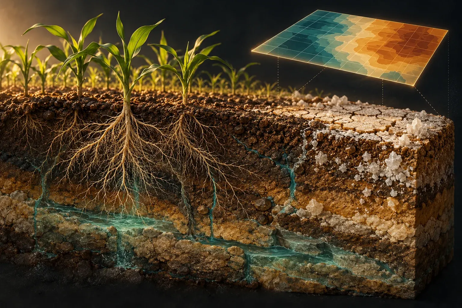
New salinity maps can reveal overlooked risks, but a colored pixel cannot tell a farmer everything about the root zone, drainage or the consequences of moving salt elsewhere.
A warning written into the map
A map of soil salinity seems to offer an unusually direct view of an agricultural problem. The colors are continuous, the boundaries are crisp and every location appears to have an answer. It is easy to imagine a land manager selecting a field, reading a value and deciding what to do next. Yet the most important information may be the small print explaining what was predicted, how the soil was tested and which year the map represents.
A 2026 study by Mohammad Aziz Zarif and colleagues illustrates that point explicitly. The researchers modeled electrical conductivity across the European Union and United Kingdom using soil observations and environmental predictors. Their author abstract warns that the estimated area above a specified conductivity value should be interpreted as elevated predicted conductivity measured at a one-to-five soil-to-water ratio, not as a direct estimate of soils meeting a particular diagnostic classification. The map represents 2018, although the paper appeared online in July 2026. Zarif and colleagues, publication record and abstract.
That distinction is not academic housekeeping. A policy reader could otherwise turn an estimated measurement into a categorical diagnosis, or treat a recent publication as a picture of conditions on the publication date. A farmer could mistake a regional prediction for a field test. A journalist could add together numbers that describe different methods, depths or definitions and produce a total that corresponds to no defensible measurement.
This article follows an original fictional irrigation district as it evaluates a proposed salinity information service. The district, its meetings and its numerical exercises are invented. They are not a report of a real project or recommendations for a particular farm. The aim is to explain how a useful map becomes a defensible decision without pretending that a global dataset can replace local agronomic and hydrological assessment.
The district begins with a question more useful than whether the map is accurate. Accurate for what purpose, over what area, at what depth and compared with which measurement? Once those questions are explicit, the colors can become valuable evidence rather than a substitute for understanding the ground beneath them.
The global problem is real, but its totals have definitions
FAO's December 2024 announcement of its global assessment reported approximately 1,381 million hectares of salt-affected soils, about 10.7 percent of global land area. It also emphasized uncertainty arising from limited data and called attention to both agricultural soils and the protection of natural saline ecosystems. This article uses the issuing organization's announcement for those bounded statements; the linked full report was not accessible through the attempted route. FAO's December 2024 assessment announcement.
The fictional district's first mistake would be to treat that global total as an instruction to reclaim every place counted. A broad environmental category can contain different land uses, ecological roles and management objectives. A naturally saline habitat is not automatically a failed agricultural field. Conversely, an irrigated field developing a salt problem should not be dismissed simply because saline environments also occur naturally.
The district therefore separates description from objective. Description asks what conditions are present and how they are changing. Objective asks what the community seeks to protect or achieve in a particular place. Those may include agricultural production, water quality, habitat, infrastructure or several goals that do not align perfectly. A map can inform the description while leaving the choice among goals unresolved.
It also separates extent from severity. Counting land above a chosen boundary does not reveal the distribution of values above that boundary, the sensitivity of the crops involved or the feasibility of changing conditions. Two districts could have the same affected area and very different problems. One might contain scattered severe patches; another might have a widespread moderate condition. The response should not be inferred from area alone.
A useful public headline can still communicate scale. It should retain the category being counted, the assessment date and the main qualification. The global figure is important because it makes a large issue visible, not because it eliminates the need to understand what each local measurement represents. Broad recognition and local diagnosis serve different purposes and should be allowed to do so.
Electrical conductivity is an indicator, not a chemical inventory
Electrical conductivity is valuable partly because dissolved ions affect how a sample conducts electricity. But a conductivity value is not a list of the individual substances present. USDA NRCS's May 2014 educator guide explicitly states that electrical conductivity does not directly measure particular ions or salt compounds. It also describes influences including soil texture, moisture-related conditions, structure and measurement timing. USDA NRCS educator guide.
At the fictional district's demonstration, a vendor displays two samples with the same conductivity number. The audience is tempted to regard them as chemically equivalent. The district's laboratory adviser stops the comparison there. A shared indicator value does not establish identical composition, identical structure or identical consequences for every intended use. The number is meaningful, but it has to remain attached to its method and interpretation.
This is a general measurement lesson with unusually practical consequences. An indicator condenses information. That makes it convenient for comparison, mapping and screening, but it also means some distinctions are not retained. Before using the indicator to choose an intervention, the district needs to know which discarded distinctions could matter to that choice. Otherwise it may purchase a precise answer to the wrong question.
The district writes a simple rule for its data system: never store the number without its measurement description. The record should identify the sample preparation, unit, depth, date and relevant quality-control information. A bare column labeled salt is not sufficient. Once a method label is lost, later users may be unable to tell whether a difference reflects the soil or merely a change in how the measurement was obtained.
The same rule applies to public graphics. A compact label can name the conductivity method and link to a short explanation. The technical detail need not dominate the page, but it should not disappear. Readers should be able to discover what the color means without tracking down a separate paper or guessing which of several possible conductivity measurements was used.
Salinity and sodicity should not be merged into one badge
The district's proposed dashboard initially uses the label salt damage for every concern. That simplifies the interface by hiding an important distinction. Total soluble salts and the role of sodium in relation to soil and water properties are connected subjects, but they are not interchangeable diagnoses. An intervention chosen on the assumption that they are identical could fail to address the relevant process.
The USDA's National Irrigation Guide distinguishes conductivity measures from sodium-related assessment. Its water-quality chapter discusses reduced permeability where exchangeable sodium is excessive under relevant conditions, rather than treating total conductivity as a complete description of the problem. The opened handbook is issued September 1997; its date is stated here because an online file location does not make it a new research publication. USDA National Irrigation Guide, water-quality chapter.
For the fictional district, the distinction changes the questions asked of a laboratory and an adviser. What evidence describes the soluble-salt condition? What evidence describes sodium-related concerns? What does the soil's physical behavior show? Which measurements are necessary to decide whether a proposed management change is appropriate? The district does not turn this list into a universal recipe; it uses it to avoid making a diagnosis from a single generic badge.
The distinction also prevents a misleading success claim. Suppose an indicator moves in a favorable direction after an intervention. That is useful information about the indicator, but it does not automatically establish that every relevant soil property improved. If the project promised better infiltration, production or water quality, those outcomes need their own evidence. A measured change is not the same as confirmation of every hoped-for benefit.
In the revised dashboard, the district uses separate labeled fields rather than a blended score. If a measurement has not been made, the field says so. The interface is slightly more complex, but the complexity corresponds to a real distinction. The purpose of design is to make that distinction understandable, not to conceal it for the sake of a cleaner-looking screen.
One method's threshold is not another method's threshold
The district now encounters conductivity values from different reports. Some refer to a saturated soil extract; others describe a specified soil-to-water mixture. The unit may look familiar across the reports, yet the preparation method differs. A reader who compares the numbers without that context risks treating unlike measurements as if they were interchangeable observations of the same quantity.
An original analogy helps explain the problem without supplying an agronomic conversion formula. Imagine two laboratories measuring the concentration of a substance after preparing the same material with different amounts of liquid. Even if both instruments report the same unit, the preparation can affect the resulting concentration. Converting between methods is not justified merely because the displayed units match. It requires an appropriate relationship and evidence that the relationship applies.
The fictional district therefore bans silent conversions in its software specification. If a dataset is transformed to make it comparable with another, the transformation must be documented, its applicability explained and the uncertainty retained. A convenient default factor is not enough. The system should also preserve the original values so that a future reviewer can understand what was changed rather than receiving only the harmonized output.
Thresholds require the same care. A boundary developed for one measurement method and purpose should not be pasted onto another map because the legend needs a red category. The district asks which definition each threshold belongs to and what decision it was intended to support. Where comparability cannot be established, the maps should remain separate rather than being forced into a single ranking.
This is not an argument against combining datasets. Combining them can be extremely useful when the measurement relationships are understood. It is an argument for making harmonization an explicit scientific task rather than an invisible formatting step. A shared color scale can create an appearance of consistency more quickly than the evidence can justify it.
A sample is a place, a depth and a moment
Sarkar and colleagues' December 2024 preprint describes 162 topsoil samples collected during a nine-day period in March 2024 in coastal southwest Bangladesh, with conductivity measured using a one-to-five soil-to-water procedure. Its author abstract describes mapping and interpolation of those observations. The article is cited here as a dated sampling example, not as a continuously observed record of every depth or every season in the region. Sarkar and colleagues, 2024 preprint.
The fictional district uses that example to revise its idea of a ground-truth point. A point on a map can look timeless and dimensionless. The underlying sample is neither. It came from a particular volume of soil, collected at a particular time and processed in a particular way. Those details determine what it can support when used to train or test a prediction.
The district's first proposed map would have displayed one value for each field. The revised proposal asks whether that value represents a surface layer, a deeper layer, an average over a defined interval or a model's prediction at a specified depth. The difference matters because a single surface observation does not logically establish the condition throughout an entire profile. The map should not imply more vertical coverage than the data provide.
Time is similarly easy to flatten. A sample collected after a particular weather or management sequence should not automatically stand for the year's maximum, minimum or typical condition. A model may estimate those quantities, but the estimate needs a stated basis. The district wants its system to distinguish the observed date from the period represented by a prediction rather than storing both under one ambiguous year label.
This produces a more useful question for future sampling. What uncertainty is the next sample intended to reduce? It might address an underrepresented depth, a season with little coverage or a part of the district that differs from the training data. Sampling becomes a way to challenge the map's weak points, not simply a way to add more dots where collection is easiest.
Satellite detail does not equal soil-sampling detail
A visually sharp satellite image can make a predicted map feel equally direct. But the image and the soil estimate are different products. The image records signals sensed by the instrument; the map uses relationships among those signals, other predictors and soil observations to infer a target quantity. A finely spaced grid does not mean a soil sample was collected at every grid location.
Wang and collaborators' July 2025 primary dataset record describes global annual maps of saturated-extract conductivity and exchangeable sodium percentage from 1980 through 2024 at one-kilometer resolution. The record specifies a scale factor and a missing-data code for its files. This article inspected the dataset description, not the approximately 38-gigabyte collection, and does not claim to have independently reproduced or validated those maps. Primary global dataset record.
For the fictional district, that record illustrates two forms of precision that should not be confused. Grid spacing describes how output is organized spatially. Predictive performance describes how well estimates correspond to the relevant measurements under a validation design. A map can have small cells and substantial uncertainty, or larger cells and useful accuracy for a regional purpose. The cell size alone does not settle its suitability.
The district also adds a data-import test to its procurement process. The software must correctly handle scaling and missing values before it draws the map. A missing-data code should never appear as an extreme environmental measurement. A stored integer should not be interpreted without its scale factor. These may sound like software details, but a mistake at this stage can manufacture a dramatic environmental pattern from a file-format convention.
A responsible interface should make prediction uncertainty discoverable alongside the predicted value. It should also identify where estimates depend on conditions poorly represented in the training observations. The most useful map is not necessarily the one that colors every location with equal confidence. Sometimes a visibly qualified region is the most honest and decision-relevant part of the product.
A good model needs a difficult test
The district's vendor presents an impressive score from a random split of its data. The laboratory adviser asks whether nearby observations from the same setting may have appeared in both training and testing groups. The question does not prove the model is poor. It asks whether the evaluation resembles the actual task: making predictions in locations or conditions that were not already closely represented during fitting.
Sarkar and Ravela's April 2026 preprint on Satkhira describes combining field observations with Landsat-derived predictors, using spatial cross-validation and bootstrap uncertainty analysis. Its author abstract also distinguishes the years of collected samples from the earlier period represented by retrospective exposure maps. The work is cited as a methodological example with those stated boundaries, not as an independently audited reconstruction of every past year's soil conditions. April 2026 Satkhira preprint.
The fictional district translates the validation issue into a practical challenge. If the service will be used on an unsampled area, it should be tested in a way that sheds light on performance away from closely related training observations. If it will be used to detect change through time, it should be challenged with genuinely informative temporal comparisons. No single split of the data automatically answers every intended deployment question.
The district also asks for errors in understandable units, not just a single abstract score. It wants to know whether errors are larger in some ranges, depths or conditions. An average can conceal the very cases that matter most for a particular decision. The evaluation should therefore show relevant slices without presenting tiny subgroups as if they provided highly stable estimates.
Finally, the district asks what happens when the model encounters an unfamiliar combination of predictors. Does the system warn the user, display a broad uncertainty range or silently produce a plausible-looking number? A model that acknowledges limited support can be more useful than one that always answers with the same visual confidence. Reliability includes knowing when a prediction deserves additional local checking.
More sensors create more evidence only if their meanings are connected
A July 2025 preprint by Jafaryahya and colleagues describes conductivity-spectroscopy measurements across soil samples with varying salinity and moisture, developing a model that also accounts for frequency and soil-related properties. The author abstract reports a controlled experimental dataset, not a universally validated field instrument. It is useful here because it makes the measurement's dependence on conditions explicit. Conductivity-spectroscopy preprint.
The fictional district is considering handheld measurements, laboratory tests, remote sensing and a predictive service. The temptation is to assume that more devices automatically produce more certainty. But the devices may respond to different volumes, depths, frequencies or conditions. Their outputs become mutually informative only when the relationships among them are understood and the relevant limitations are preserved.
An original comparison makes the issue tangible. Suppose one device provides a rapid signal over a broad footprint, while a laboratory result characterizes a small collected sample. A disagreement is not automatically evidence that one device is broken. The two may be observing different supports or responding to different conditions. The district needs a comparison design that makes those differences visible before treating one as a direct substitute for the other.
The team therefore creates a measurement dictionary. Each entry names the target quantity, method, unit, spatial support, depth sensitivity and important operating conditions. Where an output is a proxy or model-derived estimate, it says so. This dictionary is a technical document, but it also protects everyday users from comparing numbers simply because the software places them in adjacent columns.
The goal is not to discourage useful new instruments. Faster measurements can help direct sampling and reveal patterns that sparse laboratory observations miss. The goal is to keep the evidential chain intact. A rapid signal, a calibrated estimate and a confirmed local diagnosis are different stages, and a well-designed service should help users move between them without quietly skipping the necessary checks.
Looking below the surface changes the investigation
A 2026 EGU conference abstract by Crabit and colleagues describes work in a southern French vineyard area combining soil sampling, geophysical measurements, surface and groundwater salinity, and water-level observations. It reports mapping at several depths and examining vegetation conditions. This is an author conference abstract, not a full independently reviewed dataset in this article, and its site-specific approach is not a universal management prescription. EGU 2026 vineyard-mapping abstract.
The fictional district takes from this example a question about investigation design rather than a ready-made answer. If the concern is movement of water and salt through a profile, which observations could distinguish competing explanations? A surface color pattern might be consistent with more than one underlying process. Additional information about depth, water levels or composition may help determine which explanation fits the place.
The district draws two invented profiles with the same surface indicator. In one, the elevated condition is concentrated near the surface. In the other, a similar surface observation overlies a different deeper pattern. The profiles are not models of the cited vineyard. They demonstrate a logical limitation: identical information at one depth does not uniquely determine the information at another.
This changes the way the district evaluates the proposed service. It no longer asks whether the map can diagnose every process from above. It asks how the map can guide a more focused investigation. A predicted hotspot might justify additional sampling; an unexpected local observation might justify revisiting the model. The relationship between mapping and fieldwork becomes iterative rather than competitive.
The distinction also improves communication with land users. A preliminary map should not be presented as a verdict that their field has a particular cause or requires a particular treatment. It can identify a reason to investigate and explain what information would make the next decision more reliable. That framing respects both the usefulness of regional evidence and the specificity of local conditions.
Salt has to go somewhere
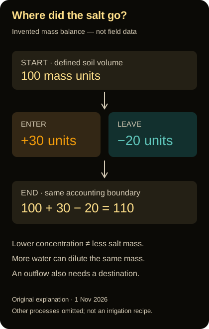
Original invented salt-mass accounting, 1 November 2026: 100 starting units plus 30 entering minus 20 leaving equals 110 units. Other processes are omitted. This is not field data or an irrigation prescription.
The district's most revealing discussion begins when someone proposes a simple success measure: lower conductivity in the sampled root-zone layer. Another participant asks where the salt would go. The question shifts attention from the condition at one location to the boundary of the management system. A local improvement may be valuable while still requiring an account of what was moved, stored or discharged elsewhere.
An original salt-accounting exercise makes the issue explicit. Begin with one hundred invented mass units of salt in a defined soil volume. During a period, thirty units enter with incoming water and other represented inputs, while twenty units leave through a specified outflow. Ignoring other processes for this deliberately simplified example, the final amount is one hundred and ten units. A balance cannot show a decrease unless the accounting includes a corresponding change in inputs, outputs or storage terms.
Now imagine that the same amount of salt is present in a larger amount of water. The concentration can be lower without the total salt mass being lower. That distinction matters when interpreting a favorable measurement after a wet period or a change in sampling conditions. The example is not a field prediction; it is a reminder to distinguish concentration, mass and the volume being described.
The district refuses to treat this exercise as a recipe for applying water. Whether additional water moves salt as intended depends on the local system, and a poorly considered intervention can create other problems. The proposed project must be assessed by qualified local specialists, including its drainage, water availability and downstream consequences. A simple accounting identity can reveal an incomplete story without telling anyone how much water to apply.
The project's reporting framework therefore contains more than a before-and-after soil value. It asks what changed in the defined soil volume, what happened to water and salt crossing the project's boundaries, and which consequences were monitored elsewhere. This is the difference between improving a sampled location and demonstrating that a management strategy is responsible at the scale where its effects occur.
Averages can hide both recovery and deterioration
The fictional district receives an annual average that appears stable. To test what stability might conceal, the team constructs a toy example with four equally weighted locations. Their initial indicator values are two, two, six and six invented units. Their later values are one, one, seven and seven. The mean remains four, although the lower-valued locations improved and the higher-valued locations worsened.
The example does not imply that real soil indicators should always be averaged this way. It shows why a summary statistic needs to be matched to a decision. A district concerned with severe local problems may need information about the distribution and location of values, not just an overall mean. A stable average is compatible with a changing pattern that matters greatly to particular land users.
Threshold counts can obscure a different distinction. If a boundary is set at five units, the number of locations above it is unchanged in the toy example. Yet their distance above the boundary has increased. Conversely, a small shift near a threshold can change the counted area sharply without representing a similarly dramatic physical change. A categorical map can make these transitions look more abrupt than the underlying values.
The team therefore proposes displaying both a continuous measure and clearly explained categories, with uncertainty where appropriate. It also distinguishes changes that are robustly supported from changes that may reflect measurement or prediction error. A small apparent difference should not become a confident trend merely because the software can subtract two grids and color the result.
For public reporting, the district chooses examples that reveal rather than hide these limitations. It explains why a map of current estimated condition differs from a map of change, and why neither alone establishes the effect of a particular intervention. This gives residents a more realistic understanding of what monitoring can accomplish and what additional evidence is required to claim success.
A management result needs a comparison
Suppose a participating field improves after a project begins. The improvement is encouraging, but the district still needs to ask what would likely have happened without the project. Weather, cropping, water supply and other conditions may also have changed. A before-and-after comparison can describe a sequence without, by itself, isolating the project's contribution.
The fictional team does not insist that every land-management decision must wait for a perfect randomized trial. Instead, it asks for a credible evaluation strategy proportional to the claim. That might include comparison areas, repeated observations, explicit accounting for important changes or a carefully justified model. Each approach has limitations, and those limitations should be stated rather than hidden behind the word impact.
The evaluation should also define success before selecting the most favorable metric. If the objective is improved production without unacceptable downstream consequences, a lower soil indicator alone is incomplete. If the objective is better diagnosis, the relevant outcome may be fewer unsupported classifications or more targeted field checks. Different projects can have different legitimate goals, but the report should not switch goals after seeing the results.
The district adds a stop-and-review provision. If monitoring reveals an unexpected adverse condition, an important assumption fails or the measurement system changes, the project should be reassessed. This is not a prediction of failure. It is an operational commitment to learning from evidence rather than defending the original plan regardless of what happens.
A mature program should be able to report mixed results. An intervention may improve one outcome, leave another unchanged and expose an unresolved concern. Those findings can guide a better next decision. Compressing them into a single success badge might satisfy a short presentation, but it would make the program less useful to the people responsible for the land and water over time.
Building a public map that does not overpromise
The district's final interface starts with three labels: what the map estimates, when it applies and what it cannot diagnose alone. A user can select a location and see the predicted value, an uncertainty description, the measurement method represented and links to relevant local observations. The interface does not display more decimal places than the evidence can meaningfully support.
Color is used carefully. The legend includes words and numerical ranges, and the page remains understandable without relying on color alone. A missing value is visibly different from a low value. An area outside the model's supported domain is not quietly filled with the same reassuring palette as an area backed by strong observations. These are not cosmetic choices; they determine whether the map communicates its limitations honestly.
The district also distinguishes access levels without concealing the science. A public regional map may be useful while precise farm-linked observations require appropriate handling and consent. The system should explain what has been aggregated and why. It should not claim that a generalized public display contains the same detail as the underlying records, nor use privacy as an excuse to omit the method and uncertainty needed to interpret the public result.
A revision panel records changes in data, methods and definitions. If a new version estimates a larger affected area, users can see whether that reflects new observations, a different model, a revised threshold or an apparent environmental change. Without this history, improvements in mapping could be mistaken for sudden deterioration, or a methodological change could be misrepresented as successful restoration.
Finally, the district offers a path from map to question. Rather than a button labeled fix this field, the page helps a user identify the relevant evidence and seek a qualified local assessment. A decision-support system should support decisions, not impersonate the complete expertise required to make them. Its value lies partly in directing attention to the next useful observation.
The cost of being wrong is part of the map's use
Before signing the contract, the fictional district tests two different uses of the same prediction. In the first, a highlighted area triggers an additional field visit. In the second, a highlighted area would automatically restrict a land-management choice. The consequences are different, so the level and kind of evidence needed cannot be assumed to be identical. A screening product can be useful without being sufficient for a more consequential determination.
The team writes down the possible errors. A false alarm could waste a sampling visit, worry a land user or lead to an unnecessary intervention if the map were used carelessly. A missed problem could delay investigation. The relative importance of those errors depends on the decision and its alternatives. There is no reason to expect one color threshold to be optimal for every user merely because it looks consistent across the website.
The district therefore separates a screening flag from a confirmed classification. The flag explains why further attention may be useful; it does not silently become a diagnosis in a downstream report. When a field visit produces new information, the system records whether the concern was supported, revised or unresolved. This gives the district a way to learn whether its screening rule actually directs resources effectively.
It also creates a route for correction. A land user can submit a relevant observation or question the applicability of a prediction without being required to prove that the entire global dataset is wrong. The district can investigate the local discrepancy while preserving the broader value of the model. Good decision support is not weakened by a correction process. It is strengthened by making disagreement observable and useful.
What the district decides to buy
The fictional district approves neither a miracle map nor an indefinite research project. It purchases a service with a bounded purpose: identify areas where further investigation is likely to be useful, maintain comparable observations and communicate change with appropriate uncertainty. The contract does not promise that satellite imagery will directly measure every root zone or prescribe a remedy for every field.
The acceptance criteria are concrete. Imported files must retain their units, scaling, missing-data conventions and versions. Model performance must be evaluated in ways relevant to the intended use. Local observations must retain depth, date and method. The public interface must distinguish prediction from measurement and uncertainty from absence of a problem. The project must preserve enough documentation for a future team to understand how each conclusion was reached.
The district also budgets for maintenance of the evidence, not just maintenance of the website. A model can become less applicable when conditions or the observing system change. New field observations can reveal weaknesses that were not obvious at launch. A service that never revisits its assumptions may remain visually polished while becoming progressively less informative.
None of this makes soil salinity a small problem. It makes the response more serious. A global assessment can reveal scale; a research map can identify patterns; a local investigation can clarify processes; a monitored intervention can test whether a chosen response works responsibly. These are complementary contributions, not interchangeable products competing to provide one final answer.
The salt map is not the soil. It is a structured claim about the soil, built from observations, methods and assumptions. The best maps make that structure visible enough that people can use them well, challenge them when necessary and improve them over time. That is how a compelling picture becomes part of a trustworthy system for protecting land, water and the livelihoods that depend on both.
Editorial and source-access note
Prepared November 1, 2026; not published. Nine distinct primary sources are cited: issuing-body guidance or assessment communication, an author dataset record, a journal author abstract, three preprint author abstracts and one conference author abstract. These have different evidential status and are not all peer-reviewed field experiments. The FAO report link and several publisher routes were unavailable; no claim of full access or independent dataset replication is made. The fictional district, numerical accounting exercises and interface proposal are original explanatory material, not advice for a particular farm. No irrigation amount, amendment dose or site-specific reclamation prescription is supplied.