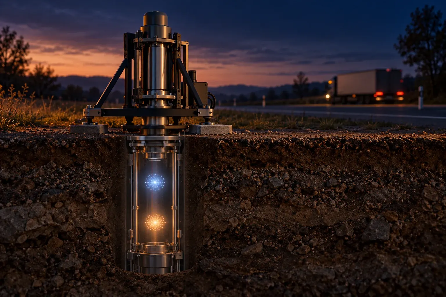
Matter-wave instruments can register extraordinarily small forces. Turning that sensitivity into a useful survey or navigation measurement requires knowing which motion belongs to the world and which belongs to the instrument.
A gravity instrument sits beside a road. Below it might be a tunnel, a water-filled layer, solid ground or some combination that a survey team has not yet resolved. Above it, a truck passes. The instrument responds. Before anyone can turn that response into a map, they must establish how much came from the underground mass distribution and how much came from motion of the apparatus itself.
This imagined scene gets to the practical difficulty behind atom-interferometer sensors. Their promise is not simply that atoms are sensitive. Sensitivity is useful only when the device can distinguish the quantity of interest from other influences that also move its reading. A powerful response to the wrong influence can make an instrument less informative rather than more.
Two primary studies published in 2026 illustrate progress at this boundary. Baynham and colleagues reported a laboratory differential interferometer that retained quantum-limited performance under deliberately imposed laser-phase noise. Their work tests a measurement principle for proposed long-baseline experiments; it does not report the detection of gravitational waves. Meister and colleagues reported a different orbital experiment measuring magnetic-field curvature inside the Cold Atom Lab. These are distinct achievements, not interchangeable demonstrations of a finished navigation system. Baynham et al., June 17, 2026; Meister et al., July 11, 2026.
Understanding what these instruments can become starts with a less glamorous question than their ultimate sensitivity: what exactly does one measurement compare? From there, the path to a useful field result passes through timing, geometry, uncertainty, environmental measurements and interpretation. The atoms are central, but they do not work alone.
A measurement needs a reference
An accelerometer does not consult a universal stationary backdrop. It compares the behavior of a test object with some physical reference. In a matter-wave instrument, atoms can provide the test object, while light and its supporting apparatus establish the interrogation reference. If that reference moves, the measurement can change even when the external quantity of interest remains constant.
The essential light-pulse picture is a controlled sequence. Light prepares a superposition of atomic motion, redirects it and allows the alternatives to interfere. The final signal is a population measurement rather than a photograph showing little objects following drawn lines. A change in relative phase alters the probabilities of the detected outcomes. This description is a simplified account of the sequence, not a statement that every atom sensor uses the same architecture. The method is laid out in the experimental discussion of Stray and colleagues' gravity-cartography work. Stray et al., experimental overview.
A helpful analogy is a comparison between two routes and a shared set of instructions. If the instructions change during the journey, the final difference can contain both route information and instruction error. The analogy does not reproduce quantum mechanics, but it makes the engineering point: the reference participates in the result.
This is why diagrams that show only a glowing atom cloud can mislead. The laser path, reference optics, timing and detection all contribute to the experiment. Removing those elements from a public illustration may be visually attractive, but it also removes the parts that explain why a quiet laboratory and a moving vehicle present different challenges.
Three questions hidden inside the word gravity
A gravimeter, a gravity gradiometer and a map of underground structure answer related but different questions. A gravimeter estimates acceleration associated with gravity under a defined measurement model. A gradiometer compares how that acceleration changes across a separation. A subsurface map interprets observations through assumptions about where material lies and how much density contrast it produces.
The dimensions already show the difference. Acceleration is measured in metres per second squared. Divide an acceleration difference by a distance and the remaining dimensions are inverse seconds squared. A gradient is not a smaller version of acceleration expressed in a more impressive unit; it is a spatial comparison.
Consider an original numerical illustration. Two hypothetical locations one metre apart differ in vertical acceleration by two billionths of a metre per second squared. Dividing by their separation gives two billionths of an inverse second squared. If the same acceleration difference occurs over two metres, the average gradient is half as large. The distance is part of the measured quantity, not an optional construction detail.
A gradient measurement can be particularly useful when a disturbance affects both locations similarly. But it does not directly announce that a particular pipe, tunnel or rock type is present. That interpretation requires a forward model and independent constraints. The distinction matters because a field operator may need a location estimate, while a physicist reports a differential phase. Several transformations stand between them, and each can add uncertainty.
Subtraction can preserve a signal while removing a disturbance

Idealized subtraction removes a perfectly matched shared contribution; mismatches leave residuals. Conceptual, not performance data.
Suppose two imaginary sensors report a useful local contribution plus the same unwanted platform motion. The first returns the local quantity at one position and the shared disturbance; the second returns the local quantity at another position and that disturbance. Subtracting their outputs removes the identical component and retains the difference between the local quantities.
The word identical carries most of the difficulty. If one channel responds a little more strongly, or samples at a different time, cancellation is incomplete. Subtraction is not a magical eraser that knows which contribution is unwanted. It removes whatever the two measurements share, including a desired signal if that signal is common to both.
The differential strategy has a long experimental history. McGuirk and colleagues' work, first submitted in 2001 and associated with a 2002 journal article, used two atom-based accelerometers in differential operation and examined disturbances from vibration and rotation. The available repository PDF carries a later generated header, which should not be mistaken for the research's original date. McGuirk et al., primary repository record and paper.
For a new deployment, the important question is therefore how closely the two channels match under the conditions that matter. Their individual readings might look terrible while the difference is useful. Conversely, each might look stable while a small mismatch corrupts the quantity obtained by subtraction. Looking only at the final differential trace can hide whether the cancellation is robust or accidentally favorable during one test.
A small mismatch can dominate a small target
Here is a deliberately simplified arithmetic case. Let the shared disturbance be one thousand units, and let the desired difference be one unit. If the channels have a relative response mismatch of one percent, the residual disturbance can be ten units. The comparison is then overwhelmed even though each channel's response differs by only a seemingly modest percentage.
Reduce that mismatch to one tenth of a percent and the residual becomes one unit, comparable with the target. At one hundredth of a percent, it becomes one tenth of a unit. These are invented normalized values, not specifications for a particular instrument. They show why a percentage that looks small in ordinary equipment can be consequential in precision measurement.
Timing mismatch creates another route for common disturbances to leak through. A rapidly changing disturbance sampled at two slightly different instants is no longer the same value in both channels. Improving amplitude matching alone cannot solve that problem. A useful validation needs to examine the frequency content and timing of the disturbances, rather than treating all vibration as one number.
The 2026 laboratory result provides a specific example of testing cancellation rather than merely assuming it. Its authors deliberately introduced phase disturbances and examined differential recovery. They also identify longer baselines and increased atom numbers as further tests, rather than claiming that their prototype settles every future scale. That boundary is part of the achievement: the experiment establishes a demonstrated regime and a concrete next question, not a universal exemption from noise.
More time can amplify both opportunity and difficulty
For a simple idealized light-pulse accelerometer, the phase response to a constant acceleration can be written in a form proportional to an effective optical wavevector, the acceleration and the square of a pulse-separation time. That scaling explains why longer interrogation is attractive. It also requires care: it describes a particular model and sequence, not every trapped, differential or multi-loop design.
As an original calculation, take an effective wavevector of ten million inverse metres, an acceleration change of one billionth of a metre per second squared and a separation time of one tenth of a second. Multiplying these values gives a phase change of one ten-thousandth of a radian. Double the time while holding everything else fixed and the phase becomes four times larger.
The attractive square does not arrive free. Atoms must remain available for interrogation and detection. The relevant light field must continue to interact with them as intended. Motion, expansion and changes in the surrounding fields can make a longer sequence more difficult to operate. The system must also account for what happens between successive measurement cycles.
This is a general engineering lesson about scaling a useful interaction. Increasing the interval over which a signal accumulates can also increase exposure to uncontrolled influences. The correct comparison is the uncertainty of the final estimated quantity under the longer sequence, not simply the size of the ideal phase. A larger signal can coexist with a worse measurement if the accompanying uncertainty grows faster.
The interval between measurements is still part of the instrument
A sensor specification often emphasizes what happens during an interrogation. A practical user also needs to know how often a usable result appears. Preparation, cooling, detection, reset and data processing can occupy time that does not contribute in the same way to the nominal measurement interval.
Imagine two fictional systems with identical uncertainty for one accepted observation. One delivers an accepted observation every second. The other delivers one every ten seconds because preparation and recovery take longer. Over a minute, they have different amounts of information even though their single-observation performance is equal. If the environment changes between observations, the slower cadence can also miss behavior that matters.
This does not mean that the faster instrument is always preferable. A slowly varying target may reward stability and low systematic error more than rapid updates. A dynamic application may demand measurements at times when a highly precise but intermittent instrument is unavailable. The application determines which trade matters.
Any statement about bandwidth should therefore identify the entire sampling process. Repeated measurements do not automatically reconstruct everything that happened in the gaps. A disturbance can vary during those gaps and influence subsequent estimates in ways that a simple average hides. A clear record includes timestamps, missing cycles and reasons for rejected observations, so that apparent quietness is not merely the absence of data.
Precision, accuracy and repeatability tell different parts of the story
An instrument can give nearly the same answer many times and still be displaced from the correct value. Repeatability describes agreement under repeated conditions. Precision concerns the spread or uncertainty associated with measurement. Accuracy concerns closeness to the quantity being sought, including systematic effects. These terms are related, but a plot of tightly grouped points does not establish all three.
Consider a hypothetical scale that always reads five units high. Averaging one hundred readings can reduce random scatter while leaving the offset untouched. A matter-wave instrument has a different physical construction, but the logical distinction remains. A statistical uncertainty that shrinks with more data is not proof that every systematic contribution has been identified.
For a field gravity measurement, some influences belong to the instrument and others belong to the environment being measured. An unwanted change in nearby mass is physically real, yet it may be irrelevant to the underground feature of interest. Calling it a systematic error can obscure the fact that the instrument may be faithfully measuring the wrong combination of sources.
A useful report separates these layers. It states how the signal was estimated, how repeat measurements behaved and which corrections or environmental assumptions entered the result. It also states what was independently checked. Agreement with another method is especially informative when that method has different dominant errors, rather than sharing the same reference or correction model.
Averaging has a condition attached
If independent random errors have a stable distribution, averaging more observations can reduce their contribution to uncertainty. In the familiar ideal case, the uncertainty of the mean decreases with the square root of the number of observations. Four times as many independent observations gives a factor of two improvement, not a factor of four.
Take a fictional measurement with a random standard deviation of eight units per observation. Sixteen independent observations would give a standard error of two units under those assumptions. Sixty-four would give one unit. These numbers are simple illustrations of the statistical relationship, not claims about any cited atom sensor.
Now suppose a slowly varying offset affects every observation collected during one session. Increasing the number of observations within that session does not create independent knowledge of the offset. The average can become extremely precise about a shifted value. Collecting data on additional days may reveal variability that a longer single session concealed.
The sensible question is how uncertainty behaves over the relevant timescales. Does it keep decreasing, flatten or begin to grow? Does the behavior persist after transport, warm-up or a change in orientation? A statement that an instrument reaches a sensitivity after a particular averaging time should preserve that time and the environmental conditions. Removing them turns a conditional measurement into an apparently permanent capability.
The laboratory can change the question rather than merely improve the answer
A device need not use free flight to make a useful matter-wave measurement. Holding atoms in an optical structure can allow a different balance of interrogation time and apparatus size. But the supporting field then becomes part of the force environment whose effects must be understood.
Panda and colleagues' June 2024 paper reports a lattice-based measurement of attraction from a small source mass and describes using signal inversions to suppress and quantify systematic effects. The complete abstract, not the subscription methods, was accessible for this article. The bounded lesson is that extended support and careful reversal can enable a useful measurement while introducing their own control problem. It is not evidence that a lattice-supported laboratory result can be transplanted unchanged into a vehicle. Panda et al., primary abstract.
A reversal is conceptually valuable because a genuine signal and an unwanted effect may respond differently when a controlled condition changes. For example, a hypothetical target signal might change sign while a detector offset remains fixed. Comparing the two conditions can separate them. But a real reversal can also alter other aspects of the apparatus, so the separation must be tested rather than assumed.
This is the difference between a clever measurement strategy and a convenient story about one. The strategy specifies what should change, what should remain fixed and how deviations will be detected. The story merely says that an error cancels. The former produces evidence; the latter risks making an untested symmetry carry the entire conclusion.
A different sequence can trade one vulnerability for another
There is no single mandatory way to extract acceleration information from atomic motion. Changing the pulse sequence changes how the instrument weights motion and disturbances. A design can become less vulnerable to one frequency range while changing its response elsewhere.
D'Amico and colleagues described a measurement based on successive velocity observations of falling atoms, using their difference to estimate acceleration. The primary preprint was submitted in March 2018, with a related journal publication in 2019. Their experiment addresses vibration sensitivity through a different measurement strategy rather than claiming that all environmental motion has ceased to matter. D'Amico et al., primary paper.
A plain arithmetic analogy helps. If two hypothetical velocity measurements are separated by two seconds and differ by six metres per second, the average acceleration over that interval is three metres per second squared. The result depends on both velocity measurements and on the interval. Errors in either observation propagate into the difference, and behavior within the interval is summarized rather than individually resolved.
The scientific value of alternative sequences is therefore broader than a competition for one best number. They offer different response functions and different checks. If two approaches agree under conditions where their dominant disturbances differ, that agreement can be informative. If they disagree, the discrepancy may help identify an overlooked influence. Diversity of measurement method can be a diagnostic resource, not merely a choice between rival products.
A road survey is an inverse problem
Return to the instrument beside the road. The team does not directly observe a tunnel with the atoms. It measures a response associated with the surrounding force field, then asks which underground arrangements could plausibly produce that response. This is an inverse problem: reasoning from observations back toward an unknown physical configuration.
The forward direction is easier to state. Given a specified density distribution, geometry and observation location, a model predicts a gravitational contribution. The inverse direction can be ambiguous because different distributions can produce similar observations at the available locations. A compact shallow anomaly and a broader deeper anomaly may not be equally distinguishable from a sparse survey.
A published field demonstration helps anchor this discussion. Stray and colleagues' February 2022 study used a gravity-gradient survey to detect a tunnel beneath a road and estimated its position through a stated inference method. That is evidence from a particular target, survey and model. Its spatial sampling and resulting position uncertainty should not be converted into a universal depth capability for every void or geological setting.
A field interpretation becomes more persuasive when it uses independent information about surface geometry, known structures and plausible materials. That information should be visible as an input, not smuggled into the result and then presented as something the sensor discovered alone. An instrument can sharply improve an investigation without being the sole source of its conclusion.
The map needs a scale and an uncertainty story
A smooth colored map can make sparse measurements look more complete than they are. Interpolation fills the space between observations according to a rule. It does not create new direct measurements there. A map of a model estimate should therefore distinguish the measured points from the reconstructed field or inferred structure.
Imagine an original survey example with five observations along a line. A smooth dip appears near the middle. Adding measurements on either side could help establish its width, while measurements along a second direction could test whether it represents a localized object or a feature extending across the site. Repeating the same line more precisely does not necessarily supply the information missing from the unmeasured direction.
The uncertainty in an inferred location can also be asymmetric. A set of observations may constrain the horizontal position more tightly than the depth, or distinguish a nearby boundary better than a distant one. Reducing the result to a single circular error symbol can erase that structure.
For readers, the most useful visualization combines the observation layout, the estimated feature and the uncertainty associated with the interpretation. It should state whether uncertainty reflects measurement noise alone or also variation in the assumed background. A model that treats the background as perfectly known can appear more decisive than the physical evidence warrants. The map's clarity should come from explaining those assumptions, not from making them invisible.
Nearby activity can be real signal and unwanted context
A force sensor responds to the world around it, including parts that the investigation did not intend to study. Nearby moving masses can change the gravitational environment. Mechanical activity can move the reference. Temperature changes can alter components or operating conditions. These pathways differ, even when they occur at the same time.
In the opening scene, the truck might therefore contribute more than one influence. A measurement strategy that suppresses reference motion does not automatically remove the gravitational effect of a nearby mass. The distinction is conceptual, not a claim that every road survey requires the same correction or that one effect dominates all others.
A good field log records relevant changes without pretending that a note alone solves them. Vehicle passages, relocation of equipment and interruptions can be compared with the measurement record. The analysis can then test whether excluding a period changes the conclusion, or whether a modeled contribution is justified. Exclusion rules should be stated, because removing inconvenient observations after seeing the answer can bias an apparently clean result.
This suggests a useful form of robustness check: repeat the inference under several defensible treatments of the uncertain context. If the main conclusion survives, the result is less dependent on one convenient choice. If it does not, that sensitivity is itself important information about what further measurements are needed.
Space removes a constraint, not every disturbance
Microgravity can extend the opportunities for manipulating cold atoms, but an orbiting laboratory is still an engineered environment. The platform has motion, equipment, fields and operational limits. A demonstration in space should be read as a measurement in that specific environment rather than as an escape from all terrestrial complications.
NASA's August 13, 2024 account describes Cold Atom Lab measurements of subtle station vibrations and remote operation of the apparatus. The agency also discusses potential future applications. Those prospects are not the same as completed measurements of Earth-wide water movement by that instrument. Keeping the original date visible avoids recasting the 2024 milestone as a new 2026 event. NASA/JPL mission account.
The later orbital magnetic-curvature study adds a different measurement capability. Its authors compare atomic states with different magnetic sensitivity and use the interferometric geometry to investigate the field within the apparatus. That result is particularly useful as a reminder that an atom sensor can be sensitive to more than the quantity featured in a headline.
For a future mission, the central question is how the complete measurement system separates contributions and connects them to the scientific target. A longer available interval is an enabling condition, not an automatic mission result. Orientation, calibration, spatial sampling and the environment around the atoms remain part of the chain from a quantum signal to a useful observation.
A navigation estimate is an accumulation of assumptions
Acceleration can be integrated over time to estimate changes in velocity, and velocity can be integrated to estimate changes in position. The same operations also accumulate errors. That is why an impressive acceleration measurement does not by itself establish a complete navigation capability.
Consider a hypothetical constant acceleration bias of one millionth of a metre per second squared. If it persists for one thousand seconds without correction, the corresponding velocity error is one thousandth of a metre per second. Under a simple one-dimensional model starting with zero error, the position error is half the bias multiplied by time squared, or half a metre. Increase the duration by a factor of ten and that particular position-error contribution becomes one hundred times larger.
These numbers are not a prediction for an actual navigation system. Real systems combine measurements, estimate changing errors and operate in more than one dimension. The example isolates why bias and duration matter. A lower noise floor and a lower long-term bias are different improvements, and an application may need both.
A navigation demonstration should consequently specify its trajectory, duration, reference information and other sensors. It should explain when external updates were available and what happened when they were not. The atom sensor's contribution can then be evaluated within the complete estimator, rather than credited with every capability of a larger system that contains it.
Orientation can turn a good sensor toward the wrong quantity
A sensitive axis measures along its orientation. If an instrument is tilted, the component of a larger acceleration projected onto that axis can change. An accurate estimate of one component may therefore require an accurate description of orientation as well as acceleration.
As a purely geometrical illustration, a small rotation can project part of a large background into a nominally transverse measurement. The relevant error depends on the geometry and which component is being estimated; it should not be summarized by one universal tilt penalty. The point is that a strong background and a small angular uncertainty can interact to produce a consequential contribution.
Rotation can also influence the trajectories and effective comparison within an interferometer. A field evaluation must therefore state more than whether the device was physically transported. Was it measured while stationary after settling, or while moving? What orientation information was available? Were the reference and atom trajectories represented consistently in the analysis?
These details explain why mobile can mean several different things. An instrument moved between stationary survey points has a different task from one continuously estimating motion aboard a vehicle. Both can be valuable. Treating the first as proof of the second skips the conditions that make the measurements interpretable.
A useful demonstration includes the unsuccessful intervals
Research papers appropriately emphasize a demonstrated result, but deployment decisions also depend on the conditions under which measurements were unavailable or rejected. An instrument that occasionally produces excellent data may serve a laboratory study well while struggling with a task that requires continuous coverage.
An original reporting example makes the issue concrete. Suppose a fictional instrument completes ninety out of one hundred scheduled measurement periods. If the ten missing periods coincide with the strongest motion, the accepted data do not represent the full operating environment. Reporting only the accepted periods can exaggerate readiness for a dynamic application.
This is not a reason to count every rejected observation as a failure of the science. Quality controls are necessary. It is a reason to report the selection process and distinguish the precision of accepted measurements from the availability of measurements. The two quantities answer different questions.
A mature evaluation can classify interruptions: planned calibration, loss of signal, environmental excursions, processing failures or other causes. Those categories help determine whether improvement requires a different optical design, better environmental tolerance or simply a change in operating procedures. They also prevent a single overall availability percentage from concealing a problem concentrated in the exact condition the user cares about most.
A fringe is periodic, while the world keeps moving
An interference signal is periodic in phase. That is scientifically useful, but it also means a measured population does not always identify one unique phase without additional information. Several possible phases can produce the same observed population. A measurement model must establish which operating region or sequence of observations resolves that ambiguity.
An original analogy is the hand of a clock. Seeing it at the top tells you an angular position, but not how many complete turns occurred before you looked. A stream of observations can help track the motion if changes between observations are sufficiently constrained. If the hand moves unpredictably through several turns during a gap, the missing history cannot be recovered from its final position alone.
The analogy has limits: an atom interferometer's detection statistics and controls are not a clock dial. But it explains why large disturbances can present more than a larger error bar. They can make the mapping from a measured outcome back to an estimated quantity ambiguous. Auxiliary information, controlled phase changes or a suitable differential analysis may help resolve the ambiguity, depending on the instrument.
This also separates dynamic range from fine sensitivity. An instrument may distinguish tiny changes around a well-characterized operating point yet have difficulty identifying a large unknown change. Reporting the smallest resolved signal without the allowed operating range leaves the reader unable to judge whether the device can follow the intended environment. Conversely, a wide range with modest resolution can be useful for establishing the coarse context within which a more sensitive measurement operates.
Designing a survey around the information it needs
A field campaign has a finite time budget. Spending longer at each point can reduce some random uncertainty, while visiting more points can reveal spatial structure. Those are different ways of improving the investigation, and the best balance depends on what is uncertain about the target.
Consider a fictional campaign with four hours of measurement time, excluding travel and setup. The team could spend an hour at each of four locations, or fifteen minutes at each of sixteen. Under an ideal independent-noise model, the longer dwell would reduce the random uncertainty at a location relative to the shorter dwell. But the denser layout might distinguish between two plausible geometries that predict similar values at the original four points. Neither plan is intrinsically superior without the question and model.
A useful planning exercise predicts observations for several plausible targets before collecting the main dataset. Where do the predictions differ most? Which additional location would discriminate between them? Which observation is mainly sensitive to an uncertain background? This approach uses the model to design an informative survey rather than waiting until afterward to discover that every point answers the same limited question.
The exercise should include realistic uncertainty and missing-data possibilities. An ideal point on a map may be inaccessible, too close to an interfering structure or unavailable during the required operating period. A robust plan identifies alternative locations and preserves enough repeated observations to check consistency. Repeating a reference location can help identify temporal changes that would otherwise be mistaken for a spatial pattern.
This reasoning connects hardware development to practical value. A reduction in measurement time can permit a denser survey, more repeat checks or a larger area, not merely a faster version of the same plot. The benefit should be described in terms of the information gained for the actual investigation. That is a more meaningful outcome than treating a lower noise figure as an end in itself.
What would make the next result more convincing?
The most informative next experiment depends on the gap in the existing evidence. If the main uncertainty is common-mode rejection, a controlled disturbance test can be more valuable than another quiet run. If the issue is transportability, repeating measurements after relocation matters. If the question is an underground interpretation, additional spatial coverage or independent geological information may be more useful than a smaller uncertainty at one point.
A strong comparison should also preserve the conventional alternative. Atom-based sensing does not need an unfairly weak baseline to be interesting. The relevant comparison asks which method provides the required information under the same practical conditions, including setup, measurement time, environment and analysis. A specialized laboratory benchmark can establish a physical advance without settling the best field workflow.
For an independent observer, the most useful questions are concrete. What quantity was estimated? What was the reference? Which disturbances were deliberately tested? Which parts of the result depend on a model rather than direct observation? How much time and operational support produced the accepted measurements? What would change the interpretation?
Those questions leave room for genuine excitement. The ability to manipulate matter waves, reject shared disturbances and operate remotely in orbit represents substantial experimental work. The excitement becomes more durable when it rests on the demonstrated capability rather than on a future application silently substituted for it.
Listening for the ground beneath the noise
The roadside instrument has no built-in understanding of tunnels, trucks or maps. It produces evidence through a carefully constructed physical comparison. The investigation supplies the model, context and tests that determine what the evidence means.
Atom interferometry's practical future therefore depends on a partnership between quantum control and ordinary measurement discipline. Longer interrogation, improved cancellation and alternative geometries can make previously difficult observations possible. Timing records, environmental checks, independent comparisons and honest uncertainty are what make those observations usable outside a carefully staged demonstration.
The right story is neither that a quantum device can see everything nor that field complications erase the value of laboratory advances. It is that each demonstrated improvement removes a particular obstacle while leaving others to be measured. A prototype can validate noise rejection. An orbital experiment can characterize a local field. A road survey can constrain an underground feature. Each result becomes more useful when its actual question remains visible.
When the truck passes, a successful instrument does not have to remain completely silent. It has to provide enough well-characterized information for the analyst to tell what happened, what can be removed, what remains uncertain and whether the ground below has actually been learned about. That is the transition from remarkable sensitivity to a measurement worth trusting.