
The planet's interior emerges from competing explanations of weak ground motions. Understanding the discoveries means following the uncertainties through the whole journey.
In September 2025, an analysis of archived InSight recordings proposed something extraordinarily specific about a place no instrument has visited: a solid inner core inside Mars. The paper by Bi and colleagues inferred a radius of 613 kilometres, with a reported uncertainty of 67 kilometres, using seismic phases that travel through the deep core or reflect from its inner boundary. That number describes the result of an inverse problem, not a ruler lowered into the planet. Its force comes from whether a proposed interior consistently explains the recorded waves. The study also acknowledges that uncertainty in three-dimensional mantle and outer-core structure could enlarge its uncertainty estimates. Bi and colleagues, September 3, 2025.
The distinction matters because an illustration of a sliced planet can make the science look finished. A bright central sphere, surrounded by clean concentric bands, appears as definite as a photograph. But the picture is the end of a chain whose beginning is a small instrument recording movement at one surface location. Between them sit event classifications, arrival picks, instrument corrections, mathematical wave propagation, mineral properties, and decisions about which possible interiors deserve comparison. The intellectually interesting object is that chain.
There is no need to diminish the discovery to explain its conditional character. Quite the reverse: the conditions show how much work the evidence is doing. A single station cannot acquire the geometry of a global network merely by recording more precisely. Yet different events send energy along different paths, and different parts of each recording respond to different structures. A limited observing system can therefore become a surprisingly rich experiment, provided that its separate pieces of information are not mistaken for independent measurements when they share the same assumptions.
The practical question for a reader is not simply whether Mars has a particular layer. It is how a layer becomes an explanation that can survive alternatives. Which part of the evidence requires a boundary? Which part estimates its depth? Which part assigns it a composition or physical state? Those are related tasks, but success at one does not automatically complete the others. A rigorous account keeps them distinguishable long enough for the reasoning to be inspected.
The station measures motion, not a cross-section
The primary instrument account published by Lognonné and colleagues in January 2019 describes SEIS as a combination of three-axis very-broadband and three-axis short-period sensors. Its design included direct deployment onto the ground and shielding against wind and temperature variations. These details explain an essential measurement ambition: obtain ground motion over complementary frequency ranges while reducing disturbances introduced by the observing system and its immediate environment. The paper is an instrument design and characterization account, not a retrospective guarantee that every recorded signal is a marsquake. The SEIS experiment paper.
Imagine, as a deliberately simplified measurement model, three terms added together in a recorded trace. One is motion generated by a distant event. Another is local motion caused by the environment. The third is the instrument's own contribution. In reality the terms can interact, and each passes through a frequency-dependent response. Nevertheless, the simple decomposition clarifies the task. Increasing the display magnification enlarges all three. A dramatic-looking wiggle is not evidence that the first term has become dominant.
Calibration translates the instrument output into an estimate of physical motion. It also tells the analyst where that translation becomes unreliable. If the instrument is much less responsive in a particular frequency band, correcting for that response can amplify small errors along with the desired signal. The useful bandwidth is therefore not established by the longest axis on a plot. It depends on signal strength, response knowledge, noise, and the question being asked.
The three spatial components carry another kind of information. They can help distinguish motion oriented in different directions. But their interpretation depends on orientation, coupling to the ground, local structure, and the character of the incoming wave. A component is a direction of measurement, not a separate station somewhere else on the planet. Treating three components as three geographically independent observations would give the experiment information it does not possess.
This is also why the surface installation belongs in the scientific story rather than only in an engineering appendix. An instrument may be exceptionally sensitive and still record the behaviour of its surroundings more strongly than the distant process of interest. Good measurements require a suitable connection to the ground and a defensible account of how local conditions alter the signal. Sensitivity and specificity are different achievements: the first makes small changes detectable, while the second helps determine what caused them.
A useful mental exercise is to ask what would happen if the same interior event occurred twice, once during a quiet interval and once during a disturbed interval. The interior would be unchanged, but the confidence of the interpretation could differ substantially. That does not make the quieter recording more real. It makes the observing conditions more favourable. An event catalogue is consequently a record of both planetary activity and the ability to recognize that activity under changing circumstances.
Noise can be the ground doing something real
Garcia and colleagues' study, first published on May 26, 2020, investigated pressure effects on the InSight seismic records. Atmospheric pressure variations can deform the ground elastically; simultaneous pressure measurements help identify and reduce the corresponding seismic contribution. Their analysis developed two decorrelation approaches and examined long-period atmospheric waves through the associated displacement. The important distinction is physical: some unwanted signal is actual ground movement driven from above, rather than a malfunction inside the seismometer. Pressure effects and seismic correction.
Calling that motion noise is a statement about the present question. For a scientist studying the atmosphere and its coupling to the surface, the same motion may be useful evidence. For an analyst looking for a weak arrival from the deep interior, it may obscure the target. There is no universal operation that separates all science from all noise. A correction selects a particular relationship between measurements and attempts to remove the contribution associated with it.
Consider an original toy example in which a recorded displacement is represented by a target signal plus twice a measured environmental variable. If the coefficient really remains two, subtracting that environmental term recovers the target in this idealized model. If the coefficient changes to three while the correction remains fixed, a residual survives. If the correction is estimated during an interval containing the target, it might mistakenly remove part of the target as well. Real analysis must therefore test where the relationship holds and what the correction does to signals with known properties.
One safeguard is to keep the before-and-after records available. Another is to assess how much an arrival changes when reasonable processing choices change. The strongest result is not necessarily the smoothest trace. A trace that has been made unusually clean can conceal the information needed to judge whether an apparent phase was introduced, shifted, or selectively preserved by the processing. Visual tidiness and evidential quality can move in opposite directions.
A frequency filter illustrates the same issue. Restricting a signal to a selected band can clarify a feature whose energy lies there. It can also change the shape and apparent timing of a pulse. The analyst must distinguish an onset identified in the raw or corrected data from the peak of a filtered waveform. Those markers need not coincide. A reported travel time should have a definition precise enough that another analyst can reproduce the pick rather than merely recognize a similar-looking bump.
Environmental correction also creates a bookkeeping requirement for uncertainty. Suppose two candidate arrivals are both adjusted using the same estimated correction. An error in that correction can move both in a related way. Their uncertainties are then partly shared. Treating them as wholly independent would overstate the amount learned by combining them. Conversely, a difference between two arrivals may cancel part of a common error. The statistical treatment should follow the physical pathway by which the error enters.
Arrival times are equations with missing terms
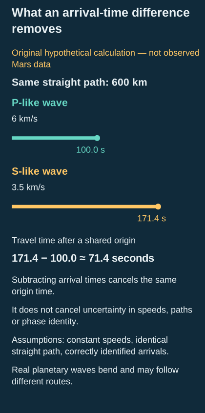
Original hypothetical calculation: a shared origin time cancels when two arrival times are subtracted. The constant-speed, same-path assumptions are deliberately simpler than real Mars seismology.
A basic travel-time equation contains an origin time and a propagation time. The clock records when energy reaches the station; the desired interior information concerns how long it travelled and along which route. If the event's start time is uncertain, a late arrival can mean a long journey, a slow medium, a late origin, or some combination. Locating the event and estimating the interior are therefore coupled problems rather than consecutive chores that can always be completed independently.
A deliberately hypothetical straight-line calculation makes the coupling visible. Let a compressional wave travel at six kilometres per second and a shear wave at three and a half kilometres per second along the same route. At a distance of 600 kilometres, their travel times would be 100 seconds and about 171.4 seconds. The separation between arrivals would be about 71.4 seconds. Subtracting the two recorded arrival times removes a shared event origin time in this toy model.
That subtraction is useful, but it does not remove uncertainty in the velocities or the path. If one adopted the wrong speed pair, the same observed separation would imply a different distance. In a layered spherical planet the paths also bend, and the two types of wave need not sample identical routes. The toy calculation explains why differential times can help; it is not an algorithm for locating actual martian events.
An observed arrival is thus better pictured as a constraint linking unknowns than as a label pinned to a known depth. Several arrivals may narrow the possibilities where their constraints intersect. But two measurements that respond to the unknowns in almost the same way may add much less information than their count suggests. What matters is the diversity of sensitivities, not simply the number of decimal places in the timing table.
Here is another original example. Suppose one measurement constrains the sum of two unknown delays to ten seconds. A second constrains the same sum to ten seconds more precisely. Precision improves, but the division between the two delays remains undetermined. A different measurement that constrains their difference would be far more valuable. Planetary interior studies face richer versions of this problem: an extra observation is especially useful when it changes the direction of uncertainty, rather than merely tightening an already measured combination.
Distance and direction deserve separate attention. Knowing that a source lies a certain distance from a station does not identify a unique surface location. On a spherical planet, the possible locations form a circle around the station until directional information or some external constraint narrows them. A beautifully estimated distance can coexist with a poorly constrained source region. A map should not convert one into the other by choosing an attractive point.
That limitation remains relevant in recent work. Dahmen and colleagues, first published January 24, 2026, analysed high-frequency marsquake recordings using an expanded catalogue and deep-learning-assisted denoising. They estimated arrival timing uncertainties and distances, but found the direction back toward the sources remained inconclusive because local resonance dominated the relevant bandwidth. Their source-region interpretation consequently remained qualified. This is a useful example of an analysis improving one coordinate of knowledge without solving all of the others. High-frequency marsquake swarms.
What a seismic boundary actually means
A wave responds to mechanical properties. A geological label is an interpretation of those properties in a physical setting. The distinction becomes important whenever a diagram assigns a crisp material boundary to a change in wave behaviour. An interface may be associated with composition, pressure-induced mineral transformation, melt, temperature, porosity, or a combination. The evidence for a change can be stronger than the evidence for one unique cause.
Knapmeyer-Endrun and colleagues' 2021 crust study, available here through its primary abstract, reported at least two and possibly three interfaces beneath InSight. Interpreting different interfaces as the base of the crust produced different local thickness estimates. Extending local seismic information with gravity and topography gave a range for global mean crustal thickness. Those are distinct inferential steps: a local interface interpretation and a planet-wide model constrained by additional observations. Neither should be presented as direct seismic sampling everywhere on Mars. The crust study's primary abstract.
To see why labels matter, imagine two hypothetical layered models. In one, a shallow contrast separates two parts of the crust and a deeper contrast marks the crust's base. In the other, the shallow contrast is the base and the deeper feature has a different explanation. Both might produce some similar arrivals. Deciding between them requires more than drawing the interfaces at their preferred depths. The model must explain the collection of observations and remain physically compatible with what is known from other measurements.
A particularly useful distinction is between resolving that a contrast exists and resolving its sharpness. A broad transition and a sharp boundary can produce similar effects at long wavelengths but different effects at shorter wavelengths. If the observations lack the relevant frequency content, a thin line in a figure may merely represent a convenient parameterization. It should not be read as evidence that nature changes abruptly over the width of that line.
The same applies to averages. A one-dimensional model summarizes properties as a function of depth. It can be an excellent description of the combinations to which the data are sensitive while leaving lateral differences unresolved. Such a model is not a claim that every point around the planet shares an identical vertical column. The proper interpretation is tied to the paths, assumptions, and smoothing used to construct it.
An original two-column example makes the averaging issue concrete. Suppose one region has a forty-kilometre layer and another a twenty-kilometre layer. An average thickness of thirty kilometres would accurately summarize equal areas, yet describe neither region individually. If the observation samples one region more strongly, even that simple average may not be the quantity inferred. A representative number needs a statement of what weighting makes it representative.
For a reader, the key question is therefore what the data resolve independently of the geological vocabulary. Does the analysis require a velocity increase? A delay? A reflector? A zone with a particular attenuation behaviour? The next question is which physical explanations can produce that feature. Keeping those questions separate makes it possible to update the geological interpretation without pretending the underlying observation has vanished.
Mineral physics supplies another set of constraints
Huang and colleagues' paper, published online October 10, 2022, interpreted triplicated compressional and shear arrivals from five events as evidence of a deep mantle discontinuity associated with a postolivine mineral transition. Their analysis connected its depth and waveform character to possible mantle temperatures and compositions. The work illustrates how a seismic feature becomes a thermal or chemical inference only after being compared with material behaviour under pressure. It does not amount to a thermometer or chemical sampler installed at the discontinuity. The mantle-transition study.
The general logic is an intersection of constraints. Suppose a measured feature could result from either a hotter material of one composition or a cooler material of another composition. A separate laboratory or theoretical relationship might rule out part of that trade-off. The combined answer is then stronger than either line of evidence alone, but it inherits uncertainties from both. The seismic fit should not erase the uncertainty in the material relationship used to interpret it.
A hypothetical linear example helps. Let a measured property depend on temperature and composition through the simple expression two times the temperature variable plus the composition variable. Many pairs give the same result. If a second independent property depends on temperature minus composition, the pair of equations can identify a unique solution in the ideal case. If the coefficients are uncertain, the solution becomes a region rather than a point. Adding physical constraints does not eliminate uncertainty; it changes its shape and, ideally, reduces it.
The word independent needs care here. Two material predictions may come from the same experimental calibration or computational assumptions. Their errors may therefore move together. Treating them as unrelated evidence can make a combined result appear more secure than it is. Likewise, two seismic models may share the same phase assignments. Agreement between their final pictures can be reassuring without constituting two completely separate discoveries.
Temperature, composition, and phase should also be distinguished in the language of explanation. A material can change crystal structure without becoming a different bulk chemical mixture. A change in mechanical properties does not necessarily imply melting. Conversely, a partly molten region may have complicated effective properties that cannot be summarized by choosing either an entirely solid or entirely liquid label. The model's categories need to be appropriate to the sensitivity of the observation.
This is one reason to resist a simple story in which each new study merely fills another blank layer in an otherwise fixed planet. A new material interpretation can alter how earlier arrivals are assigned, which changes the inferred geometry, which in turn changes the conditions relevant to the material model. The reasoning is iterative. Its credibility depends on whether those feedbacks are explored rather than hidden behind a single preferred cross-section.
A smaller metallic core can mean a different boundary
Two studies published on October 25, 2023, made the interpretive stakes especially clear. Khan and colleagues combined waves diffracted near the deep boundary region with calculations of iron-alloy properties, supporting a molten silicate layer above a smaller and denser metallic core. The argument changed the assignment of deep structure rather than merely adjusting an isolated numerical radius. The inferred layer and core properties arose together from the chosen model and the combined constraints. Khan and colleagues.
Samuel and colleagues developed a complementary geophysical case for an enriched molten silicate layer, considering seismic observations alongside tidal and thermal constraints. Their scenario also separated the base of the solid mantle from the boundary of the metallic core. A January 2, 2024 correction replaced an incorrectly plotted histogram and its source data; the corrected figure should be used rather than a cached original. The present discussion does not reproduce that histogram or derive a new estimate from it. Samuel and colleagues and the author correction.
The conceptual lesson is powerful because the change is topological as well as numerical. In one model, a particular interface is where solid mantle meets metallic liquid. In another, it is where solid mantle meets molten silicate, with the metallic boundary farther down. An arrival associated with a solid-to-liquid contrast does not, by that fact alone, identify the liquid's composition. Other evidence is needed to decide which physical boundary is being observed.
Imagine a hypothetical survey that detects a strong reflector beneath a layered surface. Calling it the bottom of the target formation immediately turns its depth into the formation's thickness. If it later proves to be an internal contrast, the measured travel time may remain correct while the reported thickness changes substantially. The mistake would have been to merge the observation and the geological assignment into one indivisible claim. The remedy is not distrust of reflections; it is a clear account of the interpretive step.
The consequences can propagate through an entire model. For a sphere, volume scales with the cube of radius. In an illustrative calculation unrelated to any published Mars estimate, reducing a candidate radius by ten percent reduces its volume to about seventy-three percent of the original. If the enclosed mass were independently fixed, the corresponding average density would have to rise by about thirty-seven percent. Real planetary models allow several quantities to change together, but the example shows why modest geometric revisions can carry substantial compositional implications.
It also shows why consistency checks are productive. A proposed size and density should fit the rest of the planet's constraints, not merely one family of arrivals. If a seismic interpretation demands an implausible composition under the adopted material model, the tension can motivate alternative structures. That does not prove which assumption is wrong. It identifies where the combined explanation needs examination.
Readers sometimes treat revision as a contest between an old wrong picture and a new final one. A better reading asks which observations became newly available or newly informative, and which assumption the revision relaxed. When a later model explains an earlier mismatch, it can represent a genuine gain in understanding even if important ambiguities remain. Progress consists in making the explanatory system more constrained and more accountable, not in promising that no boundary will ever move again.
Weak arrivals and the temptation of a clean stack
Some information is difficult to recognize in an individual recording but becomes more visible when multiple records are aligned and combined. The general operation is straightforward: preserve what is coherent under a proposed timing relationship while reducing contributions that vary irregularly. Its success depends on the alignment model and on how noise and source differences behave across the records. Averaging is not a machine that converts uncertainty into certainty by repetition alone.
In an idealized statistical example, suppose each record contains an identical signal plus independent, zero-mean noise of equal variance. Averaging twenty-five records preserves the signal while reducing the noise standard deviation by a factor of five. That square-root improvement depends on the independence assumption. If all records contain the same uncorrected artifact, the artifact survives the average just as the desired signal does. Repeated measurements cannot average away a shared bias.
A second risk appears when the alignment rule is selected because it makes a feature look most convincing. Searching many candidate alignments gives noise many opportunities to form a promising pattern. The appropriate comparison is not merely whether one chosen stack contains a peak. It is how often a similarly persuasive peak would arise under the full search procedure when the proposed signal is absent. The search itself belongs in the uncertainty assessment.
A useful original thought experiment is to compare two analysts. The first chooses a timing relationship in advance, constructs one stack, and evaluates a specified feature. The second tries a hundred relationships, selects the clearest peak, and reports it as though it had been specified beforehand. Even if their final plots look alike, the evidential situations differ. The second analysis needs a treatment of selection that the first does not require in the same form.
Robustness tests can ask whether a result depends overwhelmingly on one event, one processing band, or one subset of records. Removing a single event should not be expected to leave every estimate unchanged, especially with sparse data. But a dramatic shift can reveal where the leverage lies. That information helps distinguish a broadly supported feature from one whose apparent generality rests on a small number of favourable observations.
This is also where a paper's supplementary material can matter as much as its headline figure. Alternative filters, rejected phase assignments, synthetic tests, and uncertainty definitions show how the interpretation was challenged. A successful test should be described in terms of what it actually excludes. Demonstrating that one alternative fails does not establish that every conceivable alternative fails. The space of explanations remains bounded by what was considered and by the physical assumptions used to generate the tests.
Reading an uncertainty interval without overreading it
A reported uncertainty attaches to an estimate under a defined analysis. It does not automatically include every way the model could be incomplete. There may be uncertainty in arrival picking, source location, instrument response, material parameters, and the structural family itself. Some studies propagate several of these carefully. Others hold particular terms fixed so that the remaining problem can be solved. A narrow interval can be entirely legitimate while still being conditional on important choices.
The inner-core study's December 3, 2025 correction repairs a Methods reference attribution; it does not report a revised radius. The notice was checked through the publisher's indexed text, with direct-access limitations documented separately. The author correction.
For any numerical result, a reader should ask what the interval means. Is it a standard deviation, a confidence interval, a posterior credible interval, or simply a range across selected acceptable models? Those constructions answer different questions. Even within one construction, the chosen probability level matters. An interval should not acquire a familiar ninety-five-percent label merely because that convention is common elsewhere.
A hypothetical pair of model families illustrates the distinction. Suppose one family gives a parameter near ten with a small conditional spread, while another gives it near fifteen with a similarly small spread. Reporting only the first family's interval makes the estimate look highly concentrated. Considering uncertainty about the family itself produces a broader or even two-peaked description. There need not be a single useful central value halfway between the peaks, especially if that intermediate value belongs to neither plausible model.
This is why the shape of the uncertainty can matter more than an extra digit. A long curved trade-off between two parameters is different from a compact cloud around one best fit. An estimator may determine one combination accurately while leaving the individual parameters poorly known. Compressing everything into separate plus-or-minus numbers can hide that structure. Where possible, the relationship between uncertain quantities should travel with the headline estimates.
Uncertainty also has an appropriate scale of language. Evidence supporting a particular boundary does not necessarily justify a detailed mineral inventory. A preferred interior can be useful for planning future observations without being a complete account of the planet. The scientific question is not whether all uncertainty has disappeared, but which conclusions remain stable when defensible alternatives are allowed to vary.
Resolution is a property of the question
A planetary cross-section encourages the eye to treat every coloured region as equally well observed. The underlying experiment rarely has that symmetry. Some combinations of depth and elastic properties may strongly affect a measured arrival, while others can vary considerably with little effect. A useful model therefore needs a description of its resolving power, not just its best-fitting parameters. The absence of visible uncertainty shading in a graphic does not make the unsampled regions precise.
An original linearized example illustrates how a hidden trade-off arises. Suppose a travel time contains contributions from two segments, one with length one hundred units and the other with length two hundred units. Small changes in their slownesses, meaning travel time per unit distance, alter the total time by one hundred times the first change plus two hundred times the second. Increasing the first slowness by twice the amount that the second decreases leaves the total unchanged. One measured time cannot distinguish those compensating changes.
Now add a second path that spends different proportions of its journey in the two segments. If its sensitivity is two hundred to one hundred rather than one hundred to two hundred, the pair can separate the changes in this idealized problem. If the second path has nearly the same proportions as the first, separation remains weak. This is the mathematical reason that diverse ray geometry is valuable. Simply measuring the same weighted average repeatedly cannot recover everything inside that average.
Actual waves also have a finite frequency content. A ray drawn as an infinitely thin line is a useful computational abstraction, not the literal width of the information collected. In a simple uniform medium, wavelength equals speed divided by frequency. For a wholly hypothetical speed of six kilometres per second and a frequency of one tenth of a hertz, the wavelength is sixty kilometres. That arithmetic does not establish a universal sixty-kilometre resolution limit: interference, bandwidth, signal quality, and the parameter being estimated all matter. It does warn against interpreting every finely drawn feature as independently resolved.
The distinction between parameter precision and spatial resolution is especially important. A model with one assumed boundary may estimate that boundary's position quite precisely because many observations constrain a single adjustable number. A model allowed to contain several nearby boundaries may have far less ability to distinguish them. Precision conditional on a simple representation is not equivalent to a detailed image of arbitrary structure. The representation itself carries information supplied by the analyst.
Regularization makes that issue explicit. In a generic inverse problem, the analyst may favour smoother solutions or penalize unnecessary complexity to prevent poorly constrained variations from dominating. Such choices can be sensible and transparent. They become misleading only when the resulting smoothness is described as though it were directly observed. A smooth preferred profile can mean that the data do not justify a rougher one, rather than that the planet is demonstrably smooth at every relevant scale.
A useful test is to ask whether a proposed feature could have been recovered if it had been present. Synthetic experiments can insert a known structure, generate predicted observations under specified conditions, and run the analysis on those observations. Recovery tests reveal something about the procedure's capability within that constructed world. They do not independently validate the assumed noise, material behaviour, or structural family. Their value depends on keeping the test's assumptions visible rather than treating a successful reconstruction as an additional observation of Mars.
The reader's most productive question is consequently quite specific: which variations would change these data enough to be distinguished? An answer to that question can be useful even when it is incomplete. It identifies where a model is informative, where it summarizes unresolved structure, and where another observation would genuinely change the situation. That is a more faithful picture of scientific resolution than counting the number of layers in the illustration.
Designing the next observation around the ambiguity
The most useful future measurement would not automatically be the one with the largest data volume. It would be one that separates explanations currently difficult to distinguish. If two models predict nearly identical signals along an existing path but different signals elsewhere, a new geometry can be worth more than many repetitions of the old one. If their predictions differ mainly in frequency dependence, improved coverage of the relevant band may matter more than another broad average.
This can be expressed without forecasting a mission. Imagine two hypothetical interior models whose predicted arrival times differ by half a second for one event geometry and by ten seconds for another. If timing uncertainty is two seconds in both cases, the second geometry is much more discriminating. The calculation is not a proposal for an actual Mars experiment; it demonstrates why observation design should target differences between plausible models rather than merely seek stronger versions of already familiar signals.
A second station would introduce genuinely new spatial information, but its value would still depend on placement, noise, timing, and which events it could record in common. A larger network is not just more instruments. It is a set of relationships among instruments and sources. Shared events can help separate source uncertainty from path effects, while varied paths can test whether a one-dimensional interior is an adequate approximation. The geometry determines which ambiguities become soluble.
Independent constraints on a source can be equally valuable. In the abstract logic of the problem, knowing where an event occurred removes some of the trade-off between location and interior structure. Knowing when it occurred helps constrain propagation time. These external facts do not make wave interpretation automatic, but they change which unknowns the seismic record must solve for itself. Information can be gained by reducing the number of unknowns as well as by adding observations.
For existing archives, better reproducibility can also create scientific value. Releasing the picks, processing parameters, response corrections, and model ensembles allows another analyst to ask a different question of the same recordings. A waveform image alone is an incomplete handover. It may show the conclusion beautifully while withholding the choices that made the conclusion possible. The reusable object is the chain from data to interpretation.
That chain should preserve unsuccessful alternatives too, at least where they explain why a preferred model was selected. A future researcher may discover that an assumption once considered reasonable deserves revision. If the old result is stored only as a polished cross-section, reassessment becomes unnecessarily difficult. If its conditional structure is retained, new evidence can be incorporated without reconstructing the entire reasoning from fragments.
The achievement of martian seismology is therefore larger than a collection of labelled layers. It is the conversion of sparse motion records into a testable account of an inaccessible world. The best account remains explicit about what was measured, what was inferred, what was assumed, and what observation could change the answer. A planet's interior becomes knowable not when the diagram stops changing, but when the reasons for changing it become increasingly precise.