
The controller that extracts energy from an ordinary swell can become the wrong controller in a storm. Wave power has to reconcile useful motion, physical limits and the electricity that actually reaches shore.
A floating machine can survive a violent sea by refusing to move very much. That sounds like an odd achievement for a device whose purpose is to extract energy from motion. It is also the central design tension of wave power. The machine must respond strongly enough to useful waves to justify its existence, yet avoid turning the largest waves into destructive excursions of its own machinery. Its behavior has to change with the sea.
CorPower Ocean's February 27, 2024 commissioning account described its C4 converter switching between tuned energy capture and a detuned survival state during an Atlantic demonstration. The developer reported limited machinery response during storms and renewed electricity export afterward. This is a dated first-party account of that campaign, not independent certification of a commercial fleet or evidence of subsequent annual production. The distinction between operating states is more instructive than the announcement's promotional language. CorPower C4 commissioning account
A more recent milestone concerns the place where such claims can be tested. On September 1, 2026, the US Department of Energy reported the August 27 opening of PacWave South, an offshore, grid-connected wave-energy test facility. Its account said operators were preparing inaugural device tests. An opened test facility and an arrangement to receive future test electricity are important infrastructure, but they are not themselves measurements of a converter's output. DOE announcement of PacWave South's opening
Together these events frame the engineering question. How does a wave machine turn a changing, oscillatory input into useful electricity without allowing the pursuit of energy to destroy its ability to operate? Answering requires following forces, timing, conversion losses, unavailable hours and uncertainty. A dramatic photograph of a buoy in a storm answers remarkably few of those questions.
The water is oscillating; the useful work needs a reference
A buoy riding a wave is not automatically generating electricity. If every relevant part moves together, there may be little relative motion across the mechanism that extracts work. A converter needs a relationship between moving bodies, between a body and an anchor or support, or between changing water pressure and a conversion device. The reference can itself move. What matters is the motion and force across the power take-off.
Consider an original hypothetical with two vertical positions, x for an upper float and y for a lower reaction body. The useful stroke is x minus y. If both move upward by one meter together, their relative displacement has not changed. If the float moves upward while the reaction body moves downward, the relative stroke can be larger than either body's individual movement. Watching only the visible surface buoy can therefore misrepresent what its machinery experiences.
The corresponding instantaneous mechanical power is force multiplied by relative velocity, with a consistent sign convention. A large force at zero relative velocity produces no instantaneous mechanical work at that interface. A large displacement reached slowly need not imply high power. These elementary distinctions are worth preserving because promotional footage emphasizes movement, while engineering measurements must follow the particular motion that passes through the converter.
A hinged multibody device poses the same question in rotational form. Torque multiplied by angular velocity gives mechanical power. The ocean can make the entire platform heave and pitch while only part of that motion contributes to useful hinge rotation. The other motion can still load structures, cables and moorings. The design is consequently more than a floating shape connected to a generator: it is an attempt to direct a complicated movement into a manageable conversion pathway.
That pathway determines which sensors matter. Position, velocity, force and electrical measurements must describe corresponding interfaces and times. Otherwise, multiplying a force from one part of the system by a velocity from another can produce an impressive number that is not a defensible energy flow. The first task is to draw the physical boundary before calculating its performance.
Timing can matter as much as the size of the movement
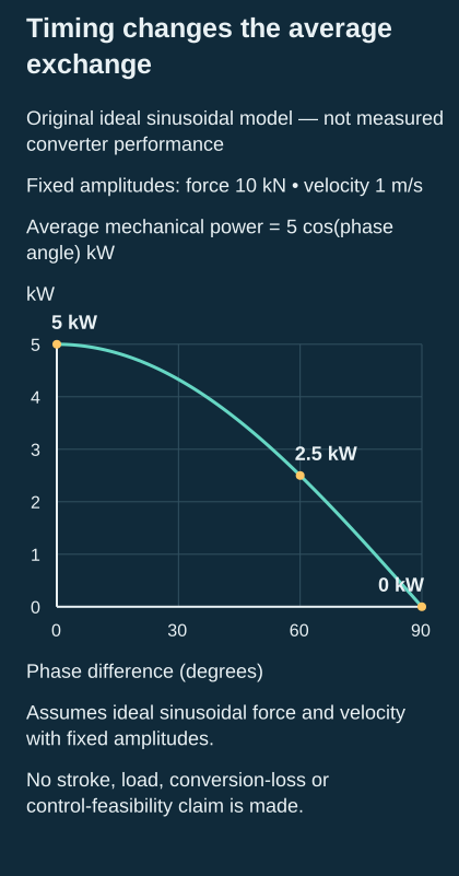
Original ideal sinusoidal calculation with fixed force and velocity amplitudes. The curve shows average mechanical exchange, not observed electricity or achievable control performance.
An original sinusoidal teaching model makes the timing issue explicit. Let an excitation force vary as F times cosinusoidal time, and let velocity vary as V times the same oscillation shifted by an angle phi. Over a complete cycle, their average product is one half of F times V times the cosine of phi. This is an ideal mathematical example, not a measured converter response or a controller specification.
If the force and velocity are aligned in this model, their average product is largest for the chosen amplitudes. If they are a quarter cycle apart, the average is zero even though both quantities remain substantial. Changing the timing can therefore change average energy exchange without simply increasing every force and every displacement. That is why control occupies such an important place in wave-energy research.
The model also reveals a trap. The amplitudes are not independent knobs that can be increased without consequence. A real machine has limits on travel, force, torque, speed, temperature and voltage. It also has hydrodynamic and mechanical relationships that change when its motion changes. An unconstrained calculation can identify an attractive phase relationship while demanding a physically impossible trajectory.
For an invented numerical illustration, take a force amplitude of ten kilonewtons and a velocity amplitude of one meter per second. Perfect alignment gives five kilowatts of average mechanical input in the ideal model. A sixty-degree phase difference gives half that average because the cosine is one half. These numbers are chosen only to expose the arithmetic. Neither case tells us the electrical output, the required stroke, the component stress or whether the motion is feasible.
The practical objective is therefore conditional: obtain beneficial timing within the machine's actual operating envelope. A controller that appears inferior in an unconstrained simulation may be more useful when its competitor repeatedly hits a travel limit. The waveform matters, but so does what the waveform asks the hardware to do.
Sometimes energy must move backward inside the machine
A simple resistive arrangement opposes motion and extracts energy as the device moves. More elaborate control may temporarily return stored energy to influence the motion before recovering more later. This can improve an idealized mechanical exchange, but it makes the distinction between gross absorbed energy and net delivered energy essential.
Imagine a hypothetical cycle in which a mechanism receives one hundred units of mechanical energy during favorable intervals and returns thirty units during other intervals. Its net mechanical absorption is seventy units. Reporting only the hundred would conceal the return flow. If conversion losses occur in both directions, the final electrical balance can be smaller again. The appropriate quantity is the signed integral over the relevant boundary, not the sum of positive peaks.
The storage involved need not be a large grid battery. It may be associated with mechanical, hydraulic, pneumatic or electrical components. Each has limits on energy, power and cycling. A component that stores enough energy for one purpose may be unable to exchange it quickly enough for another. Energy capacity and instantaneous power capacity are separate specifications.
The 2019 Wave Energy Converter Control Competition overview compared controllers on a shared numerical point-absorber problem informed by tank measurements. Its evaluation considered converted power and physical-limit use, and it distinguished that simulation stage from subsequent experimental implementation. The paper is valuable as a controlled comparison framework, not proof that its simulated rankings transfer unchanged to an ocean deployment. Ringwood and colleagues, control competition overview
For a reader evaluating a control claim, three boundaries deserve separate answers. How much energy crossed from water to moving structure? How much reached the electrical conversion stage after internal exchanges? How much was exported after auxiliary consumption and other losses? A method can improve the first number while disappointing on the last. That is not a contradiction; it means a component objective was mistaken for the system objective.
One average sea state can conceal very different demands
A sea does not usually arrive as an endless sequence of identical waves. Its surface contains overlapping components with different periods and directions. A single height and a single characteristic period compress that complexity into a convenient description. Such descriptors are useful, but they do not preserve every feature relevant to a machine with frequency-dependent response and finite travel.
A deliberately simplified comparison illustrates the issue. Suppose two artificial inputs have the same total variance. One concentrates its motion near a device's strongest response frequency. The other distributes the same variance across frequencies to which the device responds weakly. The inputs share one summary statistic but need not produce the same power or loads. A response function must be combined with the distribution of input, rather than evaluated only at an average.
Direction adds another distinction. A device that responds differently along different axes can experience different useful excitation when the directional spread changes. A narrow swell aligned with a preferred axis and a crossing sea can challenge the same geometry in different ways. This does not establish which configuration is best. It establishes why a site description cannot be reduced to a single annual height.
Ulm, Huang and Cross's March 19, 2025 experiment studied a fixed oscillating-water-column model in irregular waves. They tested representative pneumatic damping through orifices and evaluated a method that used regular-wave information to estimate irregular-wave performance. The results were bounded to the investigated geometry and comparisons; the authors called for further validation across other designs. An orifice-based power-extraction estimate is also distinct from grid electricity measured through an operating turbine and generator. Fixed OWC model in irregular waves
This is a useful example of a broader experimental strategy: simplify the input enough to understand a response, then test how well that understanding survives a more complicated input. The second step is not optional decoration. Without it, a device can be optimized for the laboratory's easiest waves rather than for the sea it is intended to encounter.
A power take-off is a machine, not an efficiency multiplier
A conceptual drawing often compresses the power take-off into a box labeled generator. That shorthand hides the part of the system where irregular movement must become a controllable electrical output. The conversion path may include gears, bearings, seals, hydraulic components, electrical machines and power electronics. Its behavior can depend on the direction, speed and history of motion.
Giorgi and colleagues' 2024 paper modeled the coupled hydraulic, pneumatic and electrical power take-off of a wave converter developed for ocean research. The originating Sandia author abstract describes comparison with bench measurements and agreement under those test conditions. Only that abstract was reviewed here. It supports the importance of validating the coupled conversion model, without establishing a universal efficiency or an ocean-lifetime result. Power take-off modeling and bench validation
Consider an original arithmetic example. A hypothetical converter absorbs ten kilowatt-hours mechanically. Suppose its conversion chain delivers eight electrically, while control, cooling and other auxiliaries consume one. Net delivery is seven kilowatt-hours. A revised controller raises mechanical absorption to eleven, but conversion falls to seven and a half because the operating trajectory shifts into a less favorable region. With the same auxiliary consumption, net delivery is six and a half. Better capture has produced worse export.
A constant efficiency assumption would miss that outcome. It may still be a useful first approximation, but it should be tested where the control change moves the machine. Low-speed reversals, high loads and brief peaks can have different consequences from steady operation near a favorable point. An average efficiency taken from one duty cycle cannot automatically be assigned to another.
The same reasoning applies to heating. Losses appear somewhere, often as heat in components with limited cooling paths. A short interval of high loss may be tolerable while repeated intervals raise temperature until a protection limit intervenes. The electrical output then depends on thermal history as well as the current wave. A credible model of annual production needs the state changes that affect availability, not merely a smooth conversion curve.
The sensor can become the bottleneck
A sophisticated controller still depends on knowing what the machine is doing. If position or speed estimates arrive late, contain noise or lose their reference, the commanded force can be appropriate to an earlier state rather than the present one. In an oscillating system, timing error is a physical error, not just a data-processing inconvenience.
The Albany M4 conference abstract published on September 8, 2025 describes dry testing and early sea commissioning of an electromechanical power take-off. It reports problems with angular sensing, attention to gearbox backlash and additional verification after equipment moved into marine cabinets. The accessible conference abstract, rather than its subscription paper, supports this account. The lesson is a concrete one about implementation; it is not a fleet reliability estimate or evidence of grid delivery, since the described output served a load resistor. Albany M4 power take-off tests
An original timing example shows why a modest delay can matter. A one-second delay corresponds to one eighth of an eight-second oscillation, or forty-five degrees of phase. This is not a claimed delay in that experiment. It simply translates time into the language of an oscillatory controller. Whether a real system can tolerate a given delay depends on its design, estimation and protective behavior.
Backlash creates a different problem. When motion reverses, a mechanical gap may have to be traversed before load transfers in the opposite direction. A model that assumes an immediate, smooth relationship between positions on both sides of the transmission can then misdescribe the reversal. Improving the model may matter more than increasing the sophistication of an optimizer built on the incorrect relationship.
These details explain why a functioning tank demonstration does not eliminate the value of dry testing or commissioning. Different tests isolate different problems. A bench can examine conversion behavior repeatably. A tank can expose hydrodynamic coupling. A sea trial adds environmental variability and operational logistics. The stages are complementary because each makes some relationships easier to inspect while leaving others unresolved.
The model can be most wrong when the controller succeeds
A model built around small movements is attractive because it can be easier to calculate and use in real time. But an energy-seeking controller may deliberately encourage larger movements. The controller can therefore take the machine outside the range in which its own prediction model was most defensible. That is a technical tension, not merely a generic warning that models are imperfect.
Celesti, Ferri and Faedo's 2024 experimental study held a prototype at different equilibrium positions to investigate changes associated with its wetted geometry. They quantified model mismatch and used the resulting model family in numerical performance studies. The physical tests and the simulated performance consequences are separate parts of the evidence. The paper does not establish that one corrected model is accurate for every large-motion event. Experimental modeling uncertainty for a prototype converter
An original thought experiment starts with a linear restoring force proportional to displacement. Within a small neighborhood, that relationship may approximate a more complicated curve well. Farther away, the actual immersed shape and restoring behavior can differ. A controller that plans a large excursion using the local straight line may predict the wrong forces precisely where its motion approaches a physical limit.
The appropriate response depends on the task. One can restrict operation to a better-characterized region, use a more detailed model, estimate changing parameters, or design control that tolerates a documented range of error. Each approach has costs. Restriction can sacrifice energy. More detail can require computation and data. Adaptation can be confused by noise. Robustness can be conservative. There is no universally free correction.
A strong comparison makes these costs visible. It asks how much performance remains when the prediction is wrong by a plausible amount, and whether protective limits still hold. A controller that performs brilliantly only when the simulation reproduces its own assumptions is less persuasive than one whose behavior has been tested against discrepancies the device is likely to encounter.
Survival mode is a different job, not a disappointing power point
During an extreme event, the objective can change from extracting energy to keeping the machine within a recoverable condition. The relevant state includes much more than the visible float. Moorings, connectors, electrical insulation, seals, foundations and access arrangements can all affect whether operation resumes afterward. Low machinery motion is useful evidence about one part of that problem, not a complete inventory of survival.
For a hypothetical design discussion, compare two strategies. One maintains aggressive capture until a hard travel limit is reached. Another reduces response earlier, giving up energy during the approach to the storm. The second may deliver less during that interval while preserving more future operating time. Evaluating the strategies only by energy captured before shutdown would answer the wrong question.
The distinction between a threshold and a transition also matters. A machine cannot necessarily change state instantaneously when a forecast or sensor value crosses a line. It may need time and available power to move to a protective configuration. A successful transition depends on the preceding condition. The engineering analysis must consider whether the protective action remains feasible when communications, external power or a sensor is unavailable.
This article does not prescribe a storm-control procedure. The useful public question is what evidence supports the claimed protective state and its entry and exit. Was the state reached under representative conditions? Which quantities were measured during the event? What inspection followed? How was restored function established? A restart signal and sustained, stable production are different observations.
Repeated survival also differs from one survival. A component can remain intact while accumulating fatigue or wear. An event that leaves no obvious external damage may still change alignment, friction or insulation condition. The next ordinary sea then begins with a machine whose history matters. Reliability assessment must connect exceptional events with the less dramatic operating periods between them.
The peak is easy to photograph; energy has to be integrated
Power is a rate. Energy is its accumulation over time. This familiar distinction becomes especially important for a converter whose output can rise and fall within individual waves, change between sea states, and disappear during maintenance or protection. A peak power number cannot be converted into annual production without an operating history or a justified model of that history.
Take an original hypothetical machine that reaches one hundred kilowatts for one second. The energy in that interval is one hundred kilojoules, or about 0.0278 kilowatt-hours. A steady ten kilowatts maintained for one hour delivers ten kilowatt-hours. The much smaller power sustained over time produces far more energy. The example is deliberately simple because an eye-catching maximum can otherwise dominate interpretation.
A useful report specifies the averaging interval and the measurement point. Mechanical power at a hinge, electrical power at a generator terminal and net exported power at a grid connection are different quantities. So are a one-second maximum, a twenty-minute mean and an annual average. The unit kilowatts alone does not disclose any of these distinctions.
Negative intervals deserve attention too. If the system imports electricity for controls or motion management, those intervals belong in the net energy balance. If an auxiliary subsystem is supplied through a separate connection, omitting it can make the main export meter look more favorable. The correct accounting boundary depends on the claim, but it should include the flows necessary to deliver the claimed service.
There is also an aggregation problem. The sum of several devices' nameplate ratings is not an observed array output. Nor does a high average during selected functioning periods establish the average across the deployment. A transparent time record distinguishes active generation, protective operation, faults, maintenance, disconnection and missing measurements. Missing data are not automatically zero, but they are not automatically favorable production either.
An annual estimate is a weighted map of many conditions
One way to reason about annual output is to divide operating conditions into categories, estimate performance in each and weight those performances by how often the conditions occur. The method is intuitive: a machine that is excellent in a rare condition may deliver less annual energy than one that is moderately effective in common conditions. The challenge lies in the evidence supporting both the performance estimates and the occurrence frequencies.
Hiles, Beatty and de Andres's September 2016 study used simulated deployments to examine uncertainty in annual-energy estimates for different converter and location combinations. It found that input duration and wave-climate variability affected the estimate. These were simulation-based results, not observed annual totals from a commercial fleet; its discussion of contemporary standards also belongs to 2016. Annual energy production uncertainty using simulations
An original three-category example makes the weighting visible. Suppose a fictional site spends half its hours in conditions delivering twenty kilowatts, three tenths delivering fifty, and the remaining fifth delivering no net power. The weighted average is twenty-five kilowatts: ten from the first category and fifteen from the second. Multiplying by a non-leap year's 8,760 hours gives 219 megawatt-hours, before any additional exclusions not already represented in those category values.
Now suppose the high-output category is poorly sampled. A few favorable observations can disproportionately influence the annual estimate. Increasing measurements only in the already well-characterized low-output category may add little confidence where it matters most. The next test should target the part of the estimate that is both consequential and uncertain.
Care is required when adding availability afterward. If a performance value already includes shutdown periods, multiplying again by an availability factor can double-count the loss. Conversely, a matrix built only from normal operating intervals can overstate annual delivery if outages are never introduced. The categories and denominators must be defined before the multiplication, otherwise a tidy calculation can conceal incompatible inputs.
A repair can last longer than the repair work
Offshore availability depends on the opportunity to intervene. A failed component may require only a short replacement in a workshop, yet remain unavailable because conditions prevent safe access or towing. The delay between detecting a fault and restoring operation can therefore dominate the actual maintenance burden.
Imagine a hypothetical converter that needs six hours of hands-on work after a fault. If access is possible immediately, downtime might be close to that duration plus transport and checks. If the next suitable window arrives several days later, the same component fault produces a much longer interruption. Calling it a six-hour repair would describe labor while hiding lost service.
The energy consequence depends on what the sea would have offered during the delay. A day unavailable in low-energy conditions and a day unavailable during productive conditions have different costs. Calendar availability and energy-weighted availability answer different questions. Neither is inherently dishonest, but substituting one for the other can distort a comparison between designs.
Modularity changes the tradeoff rather than eliminating it. A removable assembly may shorten workshop work while adding connectors, lifting interfaces and handling demands. Towing a whole device ashore may reduce offshore work but interrupt generation and require a suitable transport window. The preferred arrangement depends on the failure modes, access conditions and support infrastructure, not simply on whether a promotional animation makes removal look easy.
A design review can treat maintenance as another physical pathway: fault detection, diagnosis, stabilization, access, retrieval, repair, verification and return. Each stage can introduce time or uncertainty. Measuring that pathway is valuable even before a device reaches a large fleet, because it reveals which apparently small design choices control the practical duration of an outage.
Smoothing a wave is different from supplying through a calm
Within-wave fluctuations and prolonged low-resource periods occupy different time scales. A small buffer may reduce rapid electrical variation without providing meaningful energy during a long calm. Treating all variability as one storage problem can produce misleading claims about what a particular component accomplishes.
For an original example, buffering a fifty-kilowatt surplus for ten seconds requires about 0.139 kilowatt-hours, ignoring losses and operating limits. Supplying the same fifty kilowatts for ten hours requires five hundred kilowatt-hours. The power rating is identical; the energy requirement differs by a factor of 3,600. A device that performs the first task has not thereby demonstrated the second.
The useful design question is the service required at the connection. A research instrument at sea may need reliable modest power with local storage. A grid-connected array may be allowed to vary its output but must meet connection conditions. A hybrid system may coordinate several resources. These applications assign different value to smoothing, forecastability, redundancy and energy density.
Control also interacts with smoothing. Limiting brief peaks can reduce the burden on downstream equipment, but it may change mechanical capture. Storing energy can improve the electrical waveform while adding conversion losses and another component that can fail. The net benefit depends on the complete duty cycle, not on whether the exported trace looks flatter in a selected illustration.
For a public comparison, the clearest presentation separates three records: the incoming conditions, the device's internal conversion behavior and the service delivered at the chosen boundary. A smooth final line becomes meaningful when the reader can see what was buffered, what was curtailed and what resources were required to produce it.
Capture width is a length, not a mysterious efficiency above one
Power arriving in a wave field is often expressed per unit width of wave crest. Dividing a device's captured power by that incoming power per meter produces a length: an equivalent capture width. The dimensions matter. A quantity expressed in meters is not an electrical efficiency, and a ratio formed by dividing it by a chosen device dimension inherits that geometric choice.
Here is an original dimensional example. Suppose an invented input carries twenty kilowatts per meter of crest and a device absorbs one hundred kilowatts mechanically. The equivalent capture width is five meters. If its chosen reference width is ten meters, the capture-width ratio is one half. The example says nothing about generator losses or net export; those belong to later boundaries. It also says nothing about whether ten meters is the appropriate reference for another type of converter.
The distinction is especially useful when comparing shapes. A narrow body interacting with an extended wave field is not necessarily restricted to intercepting a rectangular strip equal to its visible frontage in the manner of a solid barrier. Conversely, a broad structure may contain substantial material that does not contribute equally to useful capture. A geometric normalization can help compare a particular design family, but it should not be mistaken for a universal thermodynamic efficiency.
A fair comparison therefore retains the numerator, denominator and measurement boundary. Is the numerator absorbed mechanical power or net electrical power? Is the incoming resource measured nearby or inferred from another location? Which dimension defines the reference width? Without these answers, two percentages that look comparable may describe different relationships. Keeping the original units visible is often the quickest way to detect the mismatch.
Travel limits couple the attractive part of the cycle to the dangerous part
A controller cannot independently optimize every instant because the present movement affects the position available a moment later. A machine approaching the end of its travel has less room to respond to the next excitation. Its useful state is therefore not just current power but position, velocity and the remaining ability to change them.
For an original idealized sinusoid, displacement amplitude X and angular frequency omega imply velocity amplitude omega times X. At a fixed velocity amplitude, a longer period requires a larger displacement amplitude because omega is smaller. Take a hypothetical velocity amplitude of one meter per second. An eight-second period gives a displacement amplitude of roughly 1.27 meters; a sixteen-second period requires roughly 2.55 meters. These are simple kinematic calculations, not permissible strokes for any cited machine.
This means that an apparently modest slow swell can challenge travel differently from a faster oscillation. A controller that promises a similar velocity response across periods may demand very different motion envelopes. The design must reconcile those demands with actual clearances and with the uncertainty in predicting the next part of the wave sequence.
An end-stop event is also different from ordinary damping. A smooth model may spread deceleration over time, whereas an abrupt contact concentrates it. Even if both remove the same kinetic energy, their force histories can differ greatly. Comparing only energy totals can therefore miss a mechanically consequential difference. This is another reason that net output and extreme response should remain separate measures rather than being compressed into one attractive performance score.
A forecast has to arrive before the useful decision
Prediction can help a controller prepare for an approaching wave, but the value of a forecast depends on its lead time, accuracy and relevance to the device. A distant measurement of surface elevation is not automatically a perfect prediction of the force that will act on a moving body later. Propagation, direction and the body's own response intervene.
An original scheduling analogy is useful. Knowing that a train will arrive soon helps only if there is enough time to reach the platform. A prediction delivered after the useful action window may be accurate as a description and useless for control. Similarly, a forecast with a long nominal horizon can have little value if uncertainty grows before the device must commit to its movement.
The control question is not simply whether a forecast is accurate on average. Errors during large excursions or transitions may matter more than errors during quiet intervals. A metric dominated by easy conditions can hide the cases in which prediction quality most affects protection or energy capture. Evaluation should follow the decision that the forecast is intended to improve.
One can test this without claiming a perfect ocean model. Feed a candidate controller forecasts with documented timing errors, amplitude errors and missing updates, then compare the resulting behavior against the intended limits. These are conceptual test categories, not instructions for operating a converter. Their purpose is to distinguish an algorithm that benefits from useful preview information from one that depends on information no deployed sensor system reliably supplies.
Repeated loads deserve a different record from the largest load
The maximum observed force is important, but it does not summarize every aspect of structural duty. Repeated smaller loads, reversals and interruptions can influence wear and fatigue. Two operating strategies may share the same highest force while producing very different histories between their extremes.
Consider an invented comparison in which strategy A reaches a high load occasionally and otherwise operates gently, while strategy B approaches that load repeatedly. A maximum-value report could make them look identical. A time history would reveal different exposure. Which history is preferable depends on the components, materials and mechanisms involved; this article does not assign a fatigue life from an illustrative waveform.
The implication for control is significant. A small increase in short-term energy might be accompanied by additional reversals or more time in a demanding operating region. That increase may still be worthwhile, but the decision requires a relationship between operating duty and maintenance or replacement. Ignoring that relationship makes the controller's objective narrower than the owner's actual problem.
A useful experimental record consequently keeps both extremes and distributions. It can distinguish how often a demanding condition occurred, how long it persisted and what state preceded it. Such records help engineers examine whether a protective change reduced one burden while shifting another elsewhere. They also allow later analysis when a recovered component reveals a failure mechanism that was not the campaign's original focus.
What a convincing next deployment should reveal
The next useful evidence for wave energy is not confined to a new maximum or a larger machine. A well-documented campaign can reveal whether a device repeatedly produces net electricity across relevant conditions, changes operating state reliably and returns from maintenance without losing the behavior demonstrated before retrieval. Those observations connect component promise with a reproducible service.
A persuasive comparison begins with an explicit question. Perhaps the team wants to know whether a new controller increases net export under matched conditions without increasing damaging excursions. Perhaps it wants to know whether a modified transmission reduces losses at reversals. Perhaps the main uncertainty concerns how quickly a fault can be diagnosed and repaired. Different questions require different measurements and cannot all be answered by one capacity figure.
The evidence should preserve unsuccessful intervals as well as attractive ones. A controller that frequently falls back to a conservative mode may still be useful, but the fallback frequency belongs in its performance description. A device that survives a storm after a costly intervention has established a different capability from one that transitions autonomously. A dataset that excludes either event leaves readers unable to evaluate the actual operating proposition.
There is no need to demand that every prototype behave like a mature utility asset before recognizing progress. Early experiments are supposed to expose weaknesses. Their value increases when the weakness becomes specific: a sensing problem, a conversion loss, a modeling mismatch, a maintenance delay, or an operating limit that arrives sooner than expected. Specific limitations can guide the next design; broad declarations of success cannot.
A wave machine earns confidence by reconciling two ambitions that initially seem opposed. It must learn how to move when movement is valuable and how to decline movement when the future of the machine is worth more than the energy in the next wave. The eventual measure is neither the tallest sea endured nor the sharpest power spike. It is useful energy delivered by a machine whose behavior, losses and interruptions can be explained.