
Astronomy helps predict when tidal currents strengthen. The electricity, mechanical loads and animal encounters still depend on what happens inside a particular stretch of water.
A tide table offers something unusual in renewable energy: a future rhythm that can be calculated well in advance. It does not offer an electrical output that stays constant between one prediction and the next. A turbine in a tidal channel must work through changing speed, reversing flow, turbulent structures and the practical limits of submerged machinery. Predictability is an advantage, but its value appears only after those changes are translated into a service someone can use.
A December 3, 2025 report from the European Marine Energy Centre makes that distinction tangible. EMEC described a completed demonstration combining a tidal turbine, vanadium flow batteries and a hydrogen electrolyser. The trial included charging, direct supply, export and battery support during lower generation. Its account also identified control and battery-management improvements. This was evidence of an integrated operating demonstration, not proof that tidal generation is intrinsically constant or that every future installation will have the same economics. EMEC's originating demonstration account.
The water surrounding a turbine is simultaneously an energy resource, a source of mechanical loading and a habitat. Those roles overlap without becoming interchangeable. A measurement campaign designed to estimate electrical yield may not resolve the rapid changes that load a blade. A camera capable of recording an animal's movement may not provide an unbiased count of every encounter. The most useful project assessment connects these measurements while respecting the question each can answer.
This article concerns tidal-stream machines, which extract energy from moving water. Their engineering should not be confused with storing water behind a barrage or with harvesting the oscillatory motion of ordinary surface waves. The distinction matters because the relevant resource, structure and environmental interactions differ. A tidal-stream turbine is placed inside a moving flow that continues around, through and beyond it.
A predictable cause meets a complicated coastline
NOAA describes tides as long-period ocean waves associated with the gravitational influence of the Moon and Sun. The rise and fall observed at a coastline is one expression of that motion. Water level and current are related, but a water-level prediction alone is not a measurement of the velocity passing through a proposed rotor location. Local geometry and flow conditions have to be characterized separately. NOAA's explanation of tides.
A narrow channel offers an intuitive example. Water moving between larger regions can accelerate through a constrained passage. Yet the speed will not necessarily be the same at every depth or across the channel. Seabed shape, bends and nearby obstructions influence the distribution. An attractive surface view may therefore conceal a poor location for a particular machine, while another part of the same channel presents a very different loading environment.
The useful prediction has several layers. Astronomical timing helps identify the repeating large-scale pattern. A site model translates that pattern into local flow. Measurements test whether the model describes the region the device will occupy. A turbine model then converts the flow distribution into expected output and loading. Each layer can be good while the next remains uncertain.
Consider a hypothetical developer with an excellent forecast of when the strongest current occurs but a biased estimate of its speed at rotor depth. The timing could be right every day while the energy forecast remains wrong. Conversely, a short measurement campaign might characterize one energetic period accurately but fail to represent the longer variation. These are different shortcomings and require different additional evidence.
The practical benefit of predictability is therefore planning. It can help schedule output, anticipate quieter operating intervals and coordinate storage or flexible demand. It does not excuse a sparse resource survey. A regular clock still needs to be connected to the actual machine and the actual site.
Why the cube makes the measurement difficult
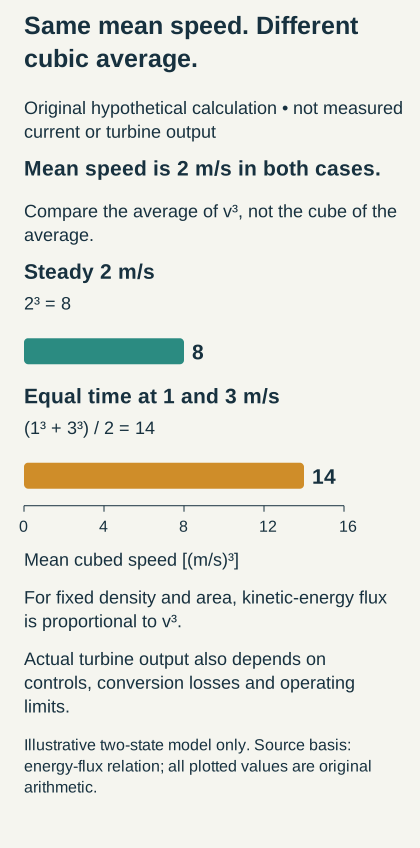
Hypothetical arithmetic, not measured resource data. With density and area fixed, averaging cubed speed differs from cubing average speed. Actual electrical output requires a device model.
The kinetic-energy flux through an area in a uniform flow scales with water density, area and the cube of flow speed. A turbine converts only part of that flux into useful power, and its controls impose additional limits. Even the elementary relationship, however, explains why a modest velocity error can become a large energy error.
As an original simplified calculation, increase a uniform current from two to three metres per second while holding everything else fixed. The cube changes from eight to twenty-seven, so the available kinetic-energy flux is multiplied by three and three eighths. That does not mean an actual turbine's electricity rises by the same factor. It may approach rated power, change its operating state or encounter conditions beyond the assumptions of the comparison.
A second example shows why averaging matters. Suppose a fictional current spends half its time at one metre per second and half at three. Its mean speed is two, whose cube is eight. But the average of the cubed speeds is fourteen. Cubing the mean would understate the average kinetic-energy flux in this artificial two-state example. Actual energy estimation should use a suitable time series and device response rather than treating one mean speed as a complete resource description.
The same issue appears across the rotor. One part of the swept area may experience faster flow than another. A single point measurement cannot automatically stand in for the area-integrated flux. The appropriate representation depends on the spatial structure and on how the rotor interacts with it. More precise measurements at the wrong location do not necessarily reduce the uncertainty that matters.
This is a good reason to distinguish a resource statistic from a power statistic. The resource may be described before installing a turbine. The power record comes from a device that alters the flow and has its own losses, limits and downtime. Both records are valuable, but they should not be merged by assuming a constant conversion factor under every condition.
The rotor sees a moving pattern, not one current speed
A blade rotates through water that varies in space and time. Even a steady vertical shear creates a changing experience for each blade as it moves between higher and lower positions. Turbulence adds fluctuations with different sizes and durations. The rotor responds to a pattern passing through its swept area, not merely to the number printed as the site's average current.
Allmark and colleagues investigated these interactions in a controlled flume campaign reported in a 2021 paper. They compared several inflow and upstream-wake configurations and used different control approaches while recording power and mechanical quantities. The results showed that operating strategy affected fluctuations and that position relative to an upstream wake mattered. These were model-scale experiments, so their numerical outcomes should not be treated as a universal full-scale loading factor. The primary power-and-loading study.
A useful mechanical distinction is between mean load and repeated load variation. Two hypothetical operating periods can have the same mean thrust while differing sharply in the number and size of fluctuations. A component exposed to repeated stress changes has a different fatigue history from one held near a constant value. An energy-only comparison can therefore miss an important part of machine life.
Imagine an invented rotor that produces the same average electrical power under two control settings. One setting permits greater speed variation and moderates some torque fluctuations. Another holds speed more tightly but transmits different fluctuations through the drivetrain. Neither is automatically better. The choice depends on the limits of blades, bearings, generator, support and electrical conversion equipment, as well as on the energy delivered.
This is why load measurements should be synchronized with operating state. A peak measured during startup, a steady generating interval and a controlled shutdown have different interpretations. Combining them into one unexplained maximum may obscure a correctable transient or an unavoidable design condition. The machine's history is part of the evidence.
Turbulence has a size as well as an intensity
A statistical description of turbulence often begins with the size of velocity fluctuations relative to a mean. That is useful but incomplete. The spatial extent of turbulent structures also matters. A fluctuation that covers most of a rotor can affect its loading differently from many smaller fluctuations distributed across the same area.
Vinod and Banerjee's 2019 primary preprint examined a model turbine under different free-stream turbulence conditions. The complete abstract describes experiments that varied both turbulence intensity and an inflow length scale, with consequences for torque variation and the near wake. This article uses that abstract's bounded description rather than inferring details from inaccessible methods. The study supports treating turbulence structure as more than one percentage attached to a site. The experimental preprint abstract.
An original analogy is to push a door in two ways. A broad push across much of its surface and several smaller alternating pushes may have the same average force while producing different motion and stress. The analogy does not model a blade, but it illustrates why spatial coherence matters. A single fluctuation statistic cannot describe every mechanically relevant feature of the forcing.
The measuring instrument also has a spatial and temporal response. Averaging over a long interval can smooth variations that remain important to a component. Sampling too slowly can miss rapid changes or misrepresent them. A useful resource campaign should therefore state which scales it resolves and which it filters out, instead of assuming that any long record is automatically a load-quality record.
There is a corresponding modeling issue. A simulation can reproduce mean speed while misrepresenting the structures that cause load fluctuations. Agreement on one average is encouraging but insufficient for a fatigue claim. Validation should match the proposed use: power prediction, peak loading and lifetime assessment may require different aspects of the modeled flow to be checked.
Ebb and flood are separate operating environments
A reversing tide invites a simple mental picture: the same flow runs backward and the turbine repeats its performance. Real sites need not be symmetric. Water approaching from one direction may have crossed different seabed features or obstructions from water approaching in the other. The device's support and neighboring equipment can also present different upstream geometries.
For a hypothetical site, suppose flood flow approaches through a relatively open reach while ebb flow emerges from a bend. Equal measured hub-height speeds would not establish equal turbulence, shear or load histories. A symmetric power assumption could then conceal a directional difference. The remedy is to preserve direction in the data and analysis rather than pooling all observations into one curve too early.
Device architecture determines how reversal is accommodated. Some arrangements change orientation or blade settings; others are designed around different directional behavior. An assessment should describe the actual arrangement rather than relying on a generic underwater-windmill image. The reversal strategy affects machinery, control transitions and the conditions during which useful output is available.
Slack water presents its own questions. Generation falls when the current is weak, but auxiliary equipment may still need power. A restart is a transition rather than an instantaneous return to rated operation. The sequence can matter for electrical integration and for animals occupying the vicinity during a stationary interval.
A yearly yield estimate should keep these states visible. Time at low current, available generating time, curtailed operation and maintenance absence should not all be grouped under a vague label of non-generation. Separating them identifies whether an improvement would come from a better rotor, different controls, storage, access planning or a change in the intended service.
One turbine changes the proposition for its neighbor
Extracting energy changes the flow downstream. A second machine may encounter a wake with reduced mean velocity and altered turbulence. At the same time, water moving around an upstream rotor can accelerate locally. The layout question involves both effects, together with the wider response of the channel.
Ouro and Nishino's 2021 primary preprint studied idealized very large arrays using theoretical analysis and numerical simulation. Its abstract describes competing wake and local-blockage effects under aligned and staggered layouts. It also explicitly excludes the larger-scale interaction between the array and natural tidal currents. That exclusion is important: a favorable modeled arrangement at a prescribed bulk flow cannot by itself establish the extractable energy of a real channel. The array study and stated scope.
The fundamental bookkeeping is simple. An array cannot be evaluated by multiplying the output of one isolated turbine by the number installed while assuming the surrounding flow never responds. Each machine changes conditions for the others, and the collection changes the resistance presented to the moving water. The degree of that interaction is site- and layout-dependent.
A hypothetical comparison makes the distinction useful. Ten isolated machines might each produce one unit under the same undisturbed reference flow. Place them close together and the array could deliver fewer than ten units because downstream machines encounter altered conditions. A revised arrangement might recover some of that difference, but the result still needs to be evaluated under the same total-system boundary. Changing the assumed incoming flow between comparisons would make the layout appear better for the wrong reason.
The strongest layout study therefore links scales. A regional or channel model establishes the relevant flow response, while a more detailed representation examines device interactions. Measurements then test whether the combined account describes reality. The objective is not the highest possible output from a conveniently located individual rotor; it is useful array performance within physical, ecological and operational constraints.
The seabed and support structure belong in the energy story
A turbine has to transfer loads somewhere. A seabed-mounted support and a floating arrangement do so differently, and both interact with the surrounding water. The support cannot be treated as an invisible accessory when assessing installation, maintenance, flow interference or environmental footprint.
Consider a purely conceptual comparison. A heavy fixed support may simplify some aspects of motion while requiring substantial offshore installation work. A floating platform may permit different access arrangements but introduces its own movement and mooring behavior. Which is preferable depends on depth, geology, current, available vessels and the machine's design. There is no reason to expect one answer across every promising channel.
Cable routing is similarly consequential. A successful rotor must deliver power through subsea and shore interfaces, and those interfaces occupy real space. The route may cross areas with different seabed conditions or other uses. A high resource estimate at one point is not yet a complete project location if the connection presents unacceptable cost, vulnerability or conflict.
An energy assessment can make these dependencies visible without turning into a construction manual. It can identify which components must be installed, inspected or recovered, what conditions permit that work and how those constraints enter expected availability. The relevant question is whether the energy estimate describes a serviceable installation rather than an ideal machine with no need for access.
This perspective also helps interpret scale. A larger rotor may capture more energy while changing lifting, support and recovery requirements. Scaling the swept area is a geometrical operation; scaling the entire offshore operation is not. A credible development pathway explains which parts become more efficient with size and which introduce new limits.
Availability should be weighted by the tide
A percentage of calendar time does not fully describe lost generation. An outage during a weak-current interval may lose little energy. The same duration during a highly productive period may lose much more. Tidal predictability makes this distinction especially relevant because the timing of expected output can inform maintenance planning.
Take an original fictional example with two one-day outages. During the first day, the device would otherwise have delivered two megawatt-hours; during the second, it would have delivered twenty. Both outages occupy the same amount of time, but their energy consequences differ by a factor of ten. A time-availability statistic would treat them equally. An energy-availability estimate would not.
The calculation requires a counterfactual: what would the machine have generated if it had been available? That estimate should use a defensible resource and performance model. It should also avoid counting external curtailment as a mechanical failure or treating every low-output interval as evidence of poor operation. The classification affects which engineering change appears valuable.
Access delays can amplify the consequences of a small fault. A component might require only a brief repair once reached, while suitable conditions for intervention take longer to arrive. Expected downtime therefore combines diagnosis, preparation, mobilization, access and repair. Reporting only hands-on repair time understates the service interruption that a project must manage.
Predictable currents can help plan an intervention, but the full access window may also depend on waves, wind and vessel limits. A favorable tidal interval is one necessary condition among several. A realistic availability model uses the overlap of those conditions, not the most favorable schedule from each considered separately.
Storage changes the shape of delivery, not the amount of free energy
The integration demonstration in the opening is useful because it treats variable generation as a system-design input. Storage can shift delivery in time, while a flexible load can change when it consumes electricity. These are different responses. A battery supplies previously stored energy; an electrolyser or another process may instead adjust its operation to the available power.
A hypothetical battery required to support a one-megawatt load for two hours must deliver two megawatt-hours, before allowing for losses and operating constraints. Its power rating must also be sufficient to supply the instantaneous demand. A large energy capacity with too small a power rating will not meet the same requirement as a smaller but more powerful system. Both dimensions belong in the comparison.
Now imagine that the low-generation interval is longer than expected or begins while the battery is only partly charged. A nameplate energy capacity does not guarantee the desired service. The operating policy must manage state of charge and decide which demand has priority. That policy may reserve capacity, curtail another use or accept interruptions according to a stated objective.
Hydrogen production introduces a conversion pathway rather than making the electrical balance disappear. Its usefulness depends on the process's operating requirements and on a real use for its output. If hydrogen is later converted back into electricity, the assessment must include both conversions and their losses. If it serves a different industrial purpose, that service should be described directly rather than counted as equivalent electrical export without explanation.
The appropriate integration design begins with the service: continuous supply, scheduled export, flexible production or some combination. Only then can the project assess whether storage, geographic diversity or demand flexibility provides the needed adjustment. Predictability makes that planning easier; it does not select the answer by itself.
Animal presence, avoidance and collision answer different questions
The ecological evidence needs the same care with definitions as the energy balance. Presence near a turbine, movement away from it, entry into the rotor region and contact with a moving blade are different observations. Each helps constrain risk, but one should not silently substitute for another.
Hastie and colleagues' study, appearing in the 2018 journal volume, examined harbour-seal responses to playback of simulated turbine sound. Its measurements supported localized avoidance of the sound under the investigated conditions. This was an acoustic-playback experiment, not direct observation of collisions at an operating turbine. It informs a potential behavioral pathway while leaving other aspects of the encounter unresolved. The primary playback study.
Avoidance can reduce the likelihood that an animal approaches moving equipment. It can also imply a change in how habitat is used. Those consequences should be examined separately rather than treating avoidance as an uncomplicated ecological benefit or harm. The significance depends on what the animal was doing, whether alternative routes or feeding areas are available and how extensive the response becomes.
An original hypothetical example helps separate the stages. Out of one thousand animals moving through a broad area, one hundred approach a device, ten enter a narrowly defined rotor vicinity and one makes contact. Those invented counts describe different conditional frequencies. A change that reduces broad-area presence is not the same as a change that improves last-moment evasion among animals already close to the rotor.
A collision-risk model needs to identify which stage each parameter represents. Otherwise a behavioral reduction could be counted twice, or a rate observed at one spatial scale could be applied at another without justification. Clearly defined states make uncertainty more tractable and reveal which observation would most improve the assessment.
An operating turbine offers a different experiment
Montabaranom and colleagues' paper, first published January 7, 2025, used multibeam sonar observations near an operating turbine in the Pentland Firth. The analysis related seal presence to operating status and environmental conditions, supporting localized avoidance during some operating conditions. The sonar observations did not distinguish the two local seal species reliably. The result is therefore evidence about the observed seals and site, not a species-specific universal response. The full operational-presence study.
A central challenge in such a comparison is that operation is not randomly assigned independently of the environment. Turbines tend to operate when currents are suitable, while animals may also change behavior with current speed, season or time of day. An analysis must consider those relationships before attributing a simple difference in counts to the machine's operation.
Imagine a hypothetical site where animals naturally visit more often during slow water. If the rotor also stops during slow water, raw counts will show more animals near a stationary machine. That pattern alone cannot tell us how much is caused by the stationary state and how much by the environmental condition associated with it. Modeling and appropriate comparisons help separate the explanations, although they do not make observational uncertainty vanish.
The spatial coverage of the sensor matters as well. A reduction inside the observed region could reflect a small route adjustment or a larger displacement. The observation is informative at its scale, and additional measurements can connect it to broader behavior. A responsible interpretation preserves that scale instead of stretching a local result into an unmeasured population outcome.
A projected track is not a three-dimensional collision
A February 3, 2026 paper by Montabaranom and colleagues examined close seal tracks from the same field campaign in more detail. It assessed collision-related factors using imaging sonar and a structured track-evaluation approach. The paper provides evidence about close encounters while preserving uncertainty in how tracks passed relative to the rotor. Because it reuses the earlier campaign, it adds a distinct analysis rather than an independent field replication. The close-track primary study.
The geometrical issue is straightforward. A path that overlaps a rotor's outline in a horizontal projection may pass above, below or through a different part of the three-dimensional volume. A two-dimensional overlap is therefore a reason to investigate an encounter, not sufficient proof of blade contact. Conversely, limited viewing geometry can make a genuinely close encounter difficult to classify.
This is analogous to two aircraft whose routes cross on a map while their altitudes differ, although the underwater sensing and animal behavior are quite different. The analogy isolates the missing coordinate. The stronger observation would resolve the dimensions and timing relevant to contact, together with the turbine's motion during the encounter.
Even a documented contact leaves a further question about consequence. Immediate motion after contact does not necessarily establish the absence of injury, and a disappearance from view does not automatically establish death. The evidence should be described at the level actually observed. This is especially important when a visually striking event becomes the centerpiece of a public argument.
A camera can record behavior without estimating an encounter rate
Cotter and colleagues' January 14, 2026 study reported optical observations around a small tidal turbine. Four fish were observed contacting the moving turbine; no seal or seabird collisions were observed in the analyzed imagery. The paper describes changing sampling approaches, imperfect fish detection and limited night coverage, and explicitly limits rate inferences. These observations are valuable behavioral evidence, but the observed counts cannot be converted into a complete deployment-wide collision probability. The full small-turbine observation study.
A general sampling example explains why. Suppose an imaginary camera records continuously during daylight but only intermittently at night. If animals and turbine operation differ between those periods, the combined recorded sample will not represent the whole day without additional information. Counting every visible event correctly does not repair the missing observation time.
Detection adds another layer. Some animals are easier to distinguish from background material than others. A movement may make an object recognizable, so the events in which an animal changes direction can be easier to identify than uneventful passage. The resulting collection can be highly informative about the mechanics of a response while being poorly suited to estimating how often that response occurs.
The right monitoring design depends on the question. High temporal resolution may be needed to resolve a brief encounter. Broader coverage may be needed to estimate presence across changing conditions. Species identification may require complementary information. A single instrument setting cannot be assumed to maximize all three goals at once.
Monitoring power and monitoring wildlife share a timing problem
An ecological observation becomes more useful when it is linked to the machine's actual state. Was the rotor moving, starting, stopping or stationary? What was the current direction? Which portions of the scene were visible? These records allow an encounter to be interpreted in its physical context rather than attached loosely to a deployment date.
The same timing discipline benefits engineering analysis. A load excursion can be compared with current fluctuations, controller action or a transition. If clocks drift or data streams have different delays, apparent cause and effect can be reversed or smeared. A synchronized record does not prove causality, but an unsynchronized one can make a sound explanation unnecessarily difficult.
For a hypothetical monitoring system, imagine one camera clock running five seconds ahead of the turbine log. An animal's approach might then be matched to the wrong operating state during a startup. Correcting that mismatch requires more than a note that both instruments were active on the same day. The time basis, known offsets and interruptions should remain recoverable in the data.
Data gaps also deserve explicit treatment. A failed instrument during the strongest currents creates a different evidence gap from a planned outage during weak flow. If the omitted conditions are those most relevant to loading or encounters, the remaining data can look reassuring for the wrong reason. Availability of monitoring and availability of generation are separate quantities that should both be documented.
Blade speed is another velocity to keep in view
The current speed and the speed of a blade tip are different quantities. For a rotating blade, the distance traveled in one revolution depends on its radius. Multiplying that distance by revolutions per second gives the tangential speed at that radius. This elementary geometry helps connect mechanical and ecological discussions without assuming that one reported water speed describes every moving part.
Consider an explicitly fictional rotor with a ten-metre radius turning at twelve revolutions per minute. Its tip travels about sixty-three metres per revolution and completes one fifth of a revolution each second. Its tangential tip speed is therefore about twelve and a half metres per second. If the incoming water moves at two metres per second, the ratio of tip speed to current speed is a little over six. These are illustrative design values, not a claim about any cited device.
A point halfway along the radius moves at half the tangential speed of the tip at the same rotation rate. An encounter near one part of a blade therefore differs from an encounter near another. The motion of the animal and water adds further geometry. A single statement that a turbine rotates slowly can be misleading when it ignores the size of the swept circle and the location being considered.
The same distinction helps explain turbine control. Rotational speed, torque and power are linked through angular velocity: mechanical power is torque multiplied by angular speed. A controller can alter that relationship as the current changes. Reading a speed trace without a torque trace leaves part of the energy conversion hidden, just as reading a torque trace alone does not establish electrical delivery.
For a hypothetical shaft carrying one hundred thousand newton-metres of torque at one radian per second, mechanical power is one hundred kilowatts. At twice the angular speed with the same torque, it is two hundred kilowatts. An actual generator and drivetrain introduce losses, and the rotor may not maintain that torque at the new speed. The calculation is a dimensional check, not a prediction that turning faster always improves the machine.
Keeping these velocities and loads separate improves communication. Resource measurements describe the approaching water. Rotor measurements describe the machinery. Animal tracks describe another moving object with its own behavior. Their interaction requires a common geometry and timeline, rather than choosing whichever one of the three speeds makes a proposed conclusion sound most reassuring or alarming.
Zero observations need an observation model
A record containing no observed collisions can be informative, but the strength of the inference depends on how many relevant opportunities were actually observed and how reliably an event would have been detected. Zero is a count within a defined observation process. It is not an automatic estimate of zero underlying risk.
An original probability exercise makes the distinction precise. Suppose there are one hundred independent, fully observed encounters, each with a hypothetical one-percent chance of a specified event. The probability of observing no events is 0.99 multiplied by itself one hundred times, about thirty-seven percent. A zero count would therefore be quite unsurprising even though the assumed event probability is not zero. This toy model does not estimate risk at any real turbine.
Now weaken the assumption that every event would be observed. Missing time, obscured views or imperfect classification make a zero count harder to interpret. The appropriate model must account for those limitations rather than quietly retaining the complete-observation assumption. More recorded hours help only to the extent that they add relevant, usable observation opportunities.
There is also a question of independence. Repeated observations of the same individual under similar conditions may not provide the same information as encounters involving different animals and circumstances. Counting tracks, individuals and observation periods answers different questions. A careful study can use each quantity, but should not switch between them merely to obtain a larger denominator.
This reasoning does not diminish a reassuring record. It shows how to strengthen one: establish the observation coverage, characterize detectability and preserve the circumstances in which the animals and machine were observed together. Then a quiet dataset can support a bounded conclusion rather than a slogan.
Choosing the next measurement before adding the next machine
A project rarely has enough time or money to measure everything equally well. The useful choice is the observation most likely to change a consequential decision. If energy yield is uncertain because rotor-depth flow is poorly characterized, another month of electrical data from a different location may contribute little. If an ecological interpretation depends on unresolved vertical position, more two-dimensional tracks may leave the central ambiguity intact.
An original planning exercise starts with competing explanations. Perhaps low output results from weaker resource, unfavorable control or mechanical unavailability. Each explanation predicts a different pattern across current, operating state and power records. The monitoring plan should be able to distinguish those patterns. Collecting a larger volume of the same ambiguous record is not necessarily progress.
For array expansion, the question changes again. Evidence from one machine can establish some component and behavioral properties, but neighboring devices alter flow and the spatial pattern of infrastructure. The next phase should test the assumptions used to extrapolate, particularly those with a large effect on yield, loading or ecological interpretation. Expansion is an opportunity to learn at a new scale, not just to repeat the original installation more often.
The test should also define what would count against the preferred explanation. A predeclared comparison can prevent a disappointing result from being redescribed as success through a new metric. That does not require rigidly ignoring unexpected findings. It requires distinguishing a planned test from a useful observation discovered along the way.
A more useful promise than constant power
Tidal-stream energy's strongest promise is a knowable rhythm connected to a useful resource. That rhythm can support scheduling, system integration and planned investigation. It does not eliminate the need to understand turbulent loading, directional differences, array feedback, offshore access or the limits of ecological observations.
The engineering goal is to convert a changing flow into a dependable service with a transparent account of the changes. A well-designed system may deliver variable electricity directly, shift some of it through storage or coordinate it with flexible demand. Its performance should be judged against that stated service rather than against an imaginary requirement that every renewable device produce an unchanging line.
The environmental goal is similarly specific: determine what animals encounter, how they respond and what consequences follow, at the relevant spatial and temporal scales. Direct observations, controlled experiments and models can contribute different pieces. Their value increases when those pieces are connected without claiming that any one of them answers the whole question.
A tidal channel will continue to look deceptively simple from shore. Water moves one way, slows and returns. Under the surface, a turbine has to negotiate a much richer sequence. The best evidence follows that sequence closely enough to tell us which part is predictable, which part is controlled, which part remains uncertain and what the next useful improvement would be.