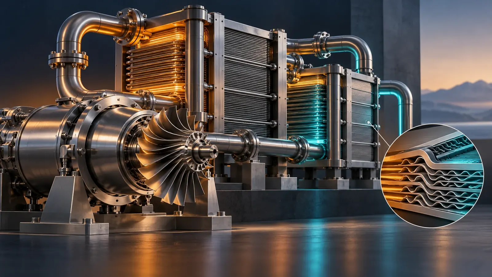
Supercritical carbon dioxide can shrink rotating machinery. Turning that advantage into reliable electricity requires an entire plant to cooperate, from microscopic flow channels to the afternoon cooling air.
The rotor is the part that makes a supercritical carbon dioxide power system easy to picture. A compact turbine spins at high speed, a generator produces electricity, and a working fluid circulates instead of being exhausted after every pass. The harder picture is the collection of heat exchangers, compressors, coolers, seals and controls that must agree on the conditions at every connection. A successful turbine can sit inside an unsuccessful power plant if those agreements are wrong.
On October 7, 2024, GTI Energy reported that the STEP demonstration plant in San Antonio had reached 27,000 revolutions per minute at a turbine operating temperature of 500°C and generated 4 megawatts of grid-synchronized electrical power. Its announcement described a later recompression configuration, a higher temperature and a 10-megawatt target as the next phase. Those were prospective statements in that dated account. The demonstrated milestone and the planned configuration should remain separate when assessing what the announcement established. GTI Energy's phase-one report.
The engineering opportunity lies in a combination of fluid properties and heat recovery. Dense carbon dioxide can carry substantial mass through relatively small passages. Compressing it near selected dense-fluid conditions can require less work than compressing a much less dense gas through a comparable pressure rise. Heat remaining after expansion can be transferred back into the high-pressure stream. Each advantage has a corresponding burden: narrow operating margins, demanding heat exchangers or a more elaborate circulation arrangement.
This is a heat engine, so its performance also depends on where the heat comes from and where the rejected heat goes. An externally heated loop could receive energy from different technologies without changing carbon dioxide into a fuel. Its environmental performance follows those technologies, the construction and operation of the plant, and losses along the way. The presence of carbon dioxide inside sealed equipment does not by itself identify the source of electricity's emissions.
A useful examination therefore follows a parcel around the loop, then asks what the parcel cannot tell us. It describes the thermodynamic states but not necessarily the stresses in the metal. It carries energy but does not reveal whether the cooling fan is consuming an excessive share of output. It passes a nominal temperature sensor while local fluid and wall conditions can differ. These distinctions explain both the attraction of the technology and the kinds of evidence needed to evaluate it.
What changes near the critical point
Carbon dioxide's critical region is conveniently close to everyday temperatures but at a pressure far above the atmosphere. NIST's Chemistry WebBook compiles critical-temperature measurements around 304 kelvin, approximately 31°C, and critical-pressure values around 74 bar, approximately 7.4 megapascals. The page includes multiple historical measurements rather than a single universal operating prescription. These approximate coordinates explain the region being discussed; a plant calculation requires an appropriate equation of state and the actual fluid composition. NIST's carbon dioxide phase data.
Above the critical temperature and pressure, a separate liquid surface and vapor phase no longer divide the equilibrium fluid in the familiar boiling-water sense. That does not make the fluid's behavior uniform. Density, heat capacity and other properties can change sharply with temperature and pressure. A diagram shaded simply as supercritical can hide a wide range of conditions, including relatively dense and relatively gas-like states.
The practical attraction of density can be understood with an intentionally simplified calculation. For a nearly incompressible fluid, reversible compression work per unit mass is approximately specific volume multiplied by pressure increase. Since specific volume is the inverse of density, doubling density would halve that simplified work estimate for the same pressure change. This is an explanatory limiting case, not a way to calculate a real near-critical compressor. Its actual work must account for changing properties, flow losses and machinery efficiency.
The same caution applies to compactness. Mass flow equals density multiplied by volumetric flow. At a hypothetical mass flow of one hundred kilograms per second, a density of five hundred kilograms per cubic metre implies a volumetric flow of one fifth of a cubic metre per second. At fifty kilograms per cubic metre, the same mass flow occupies two cubic metres per second. These deliberately chosen numbers illustrate the geometry incentive; neither pair is a specified operating point for the demonstration plant.
Less volumetric flow can reduce passage dimensions, but size cannot be scaled from density alone. Blade speed, aerodynamic loading, clearances, material stress and allowable shaft motion remain relevant. Smaller passages can make a manufacturing tolerance occupy a larger fraction of the available gap. A compact rotor may therefore exchange one kind of engineering difficulty for another rather than eliminating complexity.
Near-critical operation also makes measurement location important. A temperature measured upstream of a compressor is not necessarily the temperature at every point around its inlet or within its impeller. Accelerating flow changes local conditions. A controller may hold one measured state inside an intended envelope while a small region moves closer to a phase boundary. Designers need a spatial and dynamic understanding, not just confidence in two numbers on the control display.
The compressor chooses the rest of the day
In a closed power loop, the turbine produces work while the compressor consumes it. The electricity available outside the plant emerges after this internal bill and other losses are paid. Reducing compression work is valuable because it can increase the difference between turbine output and the machinery required to maintain circulation. Yet an advantageous design point is only one location on a compressor's operating map.
A 2022 study by Toni and colleagues reported experiments on a megawatt-scale compressor built and tested in 2021. The complete university-hosted abstract describes near-critical operation and agreement between predicted and measured performance, including a sudden choking behavior associated with phase change. The full paper was inaccessible during this retrieval, so this account does not infer unreported uncertainty or operating limits. The abstract nevertheless provides direct experimental reason to treat local phase behavior as a machinery issue. Primary author abstract for the compressor study.
A compressor map organizes quantities such as mass flow, pressure rise, speed and efficiency. These coordinates are linked. Changing a valve or altering heat rejection can move the machine away from its intended point. The plant must maintain useful output while avoiding regions where the compressor cannot provide stable or suitable operation. A nominal peak efficiency says little about the width of that usable region.
Imagine two hypothetical compressors with identical efficiency at the design point. One retains acceptable performance across a broad range of inlet temperatures and flows. The other performs better within a narrow band but requires substantial derating outside it. Which is preferable depends on the site's cooling conditions, the power demand and the available controls. A peak-value comparison would miss the decision that matters over a year.
This creates a connection between the compressor and the weather. The cooler determines how closely the working fluid can approach the available heat sink. On a warm afternoon, a dry-cooled system cannot assume the same low inlet temperature available during a cool night. Additional fan power may help move heat, but it cannot make ordinary air cooling behave as if the outdoor air were colder than it is.
The design response might involve a different operating point, lower output, a modified cycle or another cooling arrangement. Each has consequences elsewhere. Raising pressure can alter equipment requirements. Increasing heat-transfer area affects cost and footprint. Accepting lower output changes the economics of hours when electricity may be valuable. The real optimization therefore starts with a climate and duty profile, rather than selecting a compressor in isolation and adding a cooler afterward.
Instrumentation should make those connections visible. A test record that includes only turbine inlet temperature and generator output leaves too much hidden. Compressor inlet conditions, flow, electrical auxiliaries and the heat-rejection environment help explain why performance changed. Without them, a genuine improvement in one component can be mistaken for a change caused by a favorable test day.
Recovering heat without recovering the same energy twice
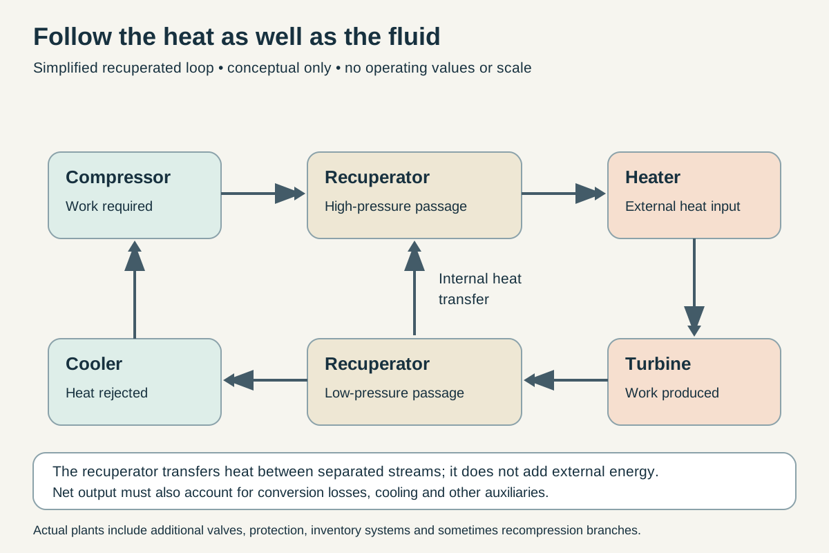
Conceptual simplified recuperated loop, not an equipment design. Heat crosses between separated recuperator streams. External heat input, heat rejection and machinery work have distinct accounting roles.
After expansion, the carbon dioxide can still be hot enough to warm the compressed stream returning toward the heater. A recuperator transfers that internal heat between the two streams while keeping them physically separate. Less external heat is then needed to reach the chosen turbine inlet state. The energy moved through the recuperator is circulating inside the plant; it should not be counted again as new heat supplied from outside.
Consider an original hypothetical energy balance. A turbine supplies one hundred units of shaft work while compression requires forty. The cycle's net shaft work is sixty units before other losses. If external heat input is one hundred and fifty units, the corresponding simplified thermal efficiency is forty percent. A recuperator that allows the same states and net work with only one hundred and twenty units of external heat would raise that illustrative ratio to fifty percent. This comparison assumes away pressure losses and other changes so that the accounting is clear.
An actual recuperator does introduce changes. Fluid loses pressure while passing through its channels. The metal has finite conductivity, and heat crosses finite temperature differences. Heat may escape to the surroundings. The streams may not divide evenly among passages. A model that improves heat recovery without charging any of these costs creates an optimistic machine that cannot be built.
The most revealing part of a recuperator can be its tightest temperature approach, often called the pinch. If the hot and cold streams approach the same temperature locally, transferring additional heat through that region becomes harder. Large total surface area does not automatically solve an unfavorable distribution of temperature differences. The entire temperature path matters, not just the inlet and outlet temperatures printed beside the drawing.
With constant heat capacities and simple counterflow, classroom temperature profiles can look conveniently straight. Real carbon dioxide may depart strongly from that picture because heat capacity varies with state. Equal mass flows on the two sides do not guarantee equal rates of temperature change as heat is exchanged. A mismatch can restrict recovery even when both streams are individually well behaved.
Recompression arrangements address this problem by dividing the flow and using more than one compression and heat-recovery path. Part of the stream can bypass the cooler before being recompressed and rejoined at a suitable location. The split changes the heat-capacity flow rates presented to parts of the recuperation system. The benefit comes from better matching, while the cost includes additional machinery, controls and integration choices.
It would be misleading to present a recompression cycle as an automatic upgrade for every heat source and climate. The useful split depends on the operating conditions and component characteristics. A configuration that looks attractive at full output might lose some advantage at part load. A comparison should therefore show the range of operation and the boundary of the calculation, rather than treating the name of the cycle as a performance guarantee.
Microscopic passages, plant-sized consequences
Printed circuit heat exchangers offer one route to compact, high-pressure heat exchange. Their flow passages can be formed in plates that are then bonded into a block. The name refers to the patterned manufacturing approach, not to an electronic circuit controlling the heat. Many narrow channels provide substantial surface area within a comparatively compact volume, while the structure has to contain the pressure difference between its streams.
Kruizenga and colleagues' 2011 experiments measured cooling heat transfer and pressure loss in small semicircular channels with supercritical carbon dioxide. Their results showed why near-pseudocritical conditions deserve special treatment: correlations evaluated using bulk properties could depart substantially from measured heat transfer, while changing how properties were evaluated improved some predictions. The experimental geometry and conditions bound the result; it is evidence for careful local modeling, not a universal correction factor for all exchangers. The original heat-transfer experiments.
A compact exchanger can be understood as a repeated local negotiation. Each channel segment must transfer enough heat without consuming too much pressure, overheating the wall or imposing an unacceptable stress. Improving one of these quantities can worsen another. Faster flow may improve heat transfer while increasing pressure loss. Thinner separating material can help conduction while reducing mechanical margin. A more elaborate passage may disturb the fluid beneficially while complicating manufacture and inspection.
At plant scale, small pressure penalties accumulate. Suppose an illustrative high-pressure stream leaves its compressor at twenty megapascals but loses half a megapascal before reaching the turbine. Another pressure loss occurs on the return side. The turbine then expands through a smaller useful pressure difference than a drawing with frictionless pipes would imply. The exact output effect requires a property model, but the direction of the penalty is already clear.
Maldistribution is another way an apparently good average can conceal a weak design. If some channels carry more flow than others, their thermal histories differ. The average outlet temperature can satisfy a specification while a portion of the block experiences a much larger temperature gradient. Designers must consider headers, manufacturing variation and transient flow distribution alongside the nominal repeated channel geometry.
The trade-off also affects maintenance. A passage that is excellent for heat transfer may be difficult to inspect or clean. A tightly integrated block can reduce joints but make an internal defect less accessible. These are not reasons to reject compact exchangers. They are reasons to evaluate a manufacturing route, inspection strategy and replacement plan together with the thermal calculation.
A useful qualification program would connect measurements at several scales. Material specimens establish relevant properties under stated conditions. Bonded samples help assess the joining process. Channel experiments test local flow and heat transfer. Larger modules expose distribution effects. An integrated loop then tests interactions with compressors and controls. Skipping from a strong small-channel result to a claim of plant readiness leaves several different questions unanswered.
The heater is a different problem from the recuperator
A recuperator exchanges heat between two branches of the working-fluid loop. The primary heater receives energy from something outside that loop. Those roles impose different requirements. The external source may be a hot solid, another fluid, combustion equipment or stored thermal energy. Its temperature range, allowable pressure, chemistry and response time influence the design of the interface.
Zhang and colleagues reported a sodium-to-carbon-dioxide prototype in March 2022. The experiment used a heat exchanger designed for fifty kilowatts of heat transfer and investigated how operating conditions affected its behavior. Its results concern a specific primary heat-transfer interface, not a complete electricity-generating plant. In particular, transferring heat at a stated rate does not establish turbine output, annual availability or an approved reactor system. The prototype experiment.
The distinction matters when comparing equipment photographs. Two compact metal blocks may have similar external dimensions while solving different problems. One faces two streams of carbon dioxide at different pressures. Another interfaces with a chemically different heat-transfer medium. A third couples the working fluid to a solid structure. Their plausible failure modes and inspection needs cannot be inferred from compactness alone.
At the March 2026 supercritical-carbon-dioxide symposium, Foster and colleagues described a sub-sized exchanger intended to inform heat-pipe microreactor coupling. The experiment used cartridge heaters, embedded temperature sensing and a carbon dioxide test facility; it was not an operating nuclear reactor. The paper reports spatial temperature measurements and pressure-loss behavior, with further higher-condition and transient testing identified as future work. Its value is component-scale evidence about how heat enters the working fluid. The 2026 primary experimental paper.
These different experiments suggest an important design question: how much of the heat source can the cycle actually use? A hot source with a large temperature decline may be poorly represented by a calculation that treats it as an infinite reservoir at one temperature. Recovering the final portion of available heat can require different equipment or operating conditions from extracting the hottest portion.
For a deliberately simplified illustration, suppose a source supplies ten megawatts of heat while cooling through two hundred degrees. Another arrangement extracts the same heat while cooling through only fifty degrees. If the source fluid's heat capacity were constant, the second arrangement would require four times the source-side mass flow. This says nothing about which complete design is better, but it identifies a burden hidden by an identical thermal-power label.
Thermal storage introduces a related issue. A storage medium's useful temperature swing helps determine how much material and circulation are needed for a given stored energy. Optimizing the power block for a narrow heat-input temperature range can affect the storage system that supplies it. The cheapest turbine arrangement need not produce the cheapest combined storage and power plant.
Ho and colleagues examined such interactions in a 2016 technoeconomic study of solar-heated carbon dioxide cycles. Their comparisons included different power-cycle configurations and the implications for solar collection and storage. The paper explicitly identified uncertain performance and cost assumptions and additional effects outside its calculation. It is a modeling study of trade-offs, not a present-day equipment quotation or measured commercial tariff. The original solar-cycle analysis.
The cooling system receives the bill
Heat rejected from the cycle is not an incidental remainder that disappears beyond the diagram. It must cross equipment into air, water or another available sink. The required temperature difference, the amount of heat and the site's resources determine the scale of that task. A highly compact turbine can still depend on a conspicuous cooling installation.
Use another hypothetical balance. A plant receives twenty megawatts of heat and exports eight megawatts of electricity. In a simplified steady state with no other energy export, roughly twelve megawatts must leave as rejected heat. Improving net efficiency reduces that burden for a fixed electrical output, but it does not remove it. The cooler has to function during the environmental conditions that matter to the plant's service.
Dry cooling avoids some water-related demands of evaporative systems, yet it requires airflow and a sufficient temperature difference to the atmosphere. The fan's electrical consumption is part of the net-power balance. A larger fan flow may lower the working-fluid temperature while drawing more power. The desirable operating point is the one that improves the whole system, not necessarily the one that produces the coldest possible measured outlet.
Boshoff and colleagues' January 2024 preprint studied a fan and air-cooled heat exchanger using computational analysis and scaled fan testing. The accessible primary abstract describes interactions between the fan, tube bundle and plenum geometry, including a trade-off involving airflow distribution. This article relies on that abstract rather than claiming to have verified every full-paper result. The study is useful because it treats cooling hardware as an interacting assembly. The fan-and-exchanger study.
Uniformity deserves attention for the same reason it matters inside a compact heat exchanger. An average air temperature or total airflow can hide regions receiving less cooling. Recirculation of warm exhaust air, obstructions or uneven flow can change the conditions seen by different parts of the equipment. A system model that assumes a uniformly supplied cooler should be tested against the layout it proposes to build.
The economics also depend on when warm conditions occur. A plant serving a demand peak that coincides with hot weather may value additional cooling capacity differently from one operating mainly at night. Annual average temperature is a weak substitute for the time series that drives both output and revenue. The relevant comparison joins meteorology, load and equipment performance hour by hour.
This is one reason headline efficiency comparisons need a specified heat-sink condition. Two systems can have different reported efficiencies because one was tested with a more favorable cooling environment. A transparent comparison either holds that condition constant or models each system under the same site profile. Otherwise, part of the apparent technology advantage may belong to the weather.
A seal can change the shape of a turbine
A rotating shaft must cross boundaries between regions at different pressures and temperatures. Seals limit leakage while allowing that motion. Their location and thermal requirements affect the length of the shaft, the placement of bearings and the arrangement of hot and cold parts. A small component can therefore influence the geometry of the entire rotating assembly.
Andretta and colleagues' 2024 dry-gas-seal paper is especially useful for its experimental boundary. Although its design ambitions reached higher conditions, the detailed conclusions describe air-helium testing with primary-seal temperatures up to 250°C and a rig-imposed speed limit of 18,000 revolutions per minute. Final tests with hotter carbon dioxide were still future work in that paper. Those distinctions prevent a designed-for condition or a short abstract statement from becoming an overstated demonstrated result. The complete seal-development paper.
Leakage has several consequences. It changes the working-fluid inventory, may require recovery or replenishment, and can carry energy away from the intended path. Depending on location, it may also influence local temperature and equipment conditions. A low leakage measurement is useful only when its pressure, temperature, working fluid, speed and duration are known.
There is a difference between preventing escape from the plant and preventing internal bypass. Fluid can remain inside the equipment boundary while bypassing a useful expansion path. That internal leakage can reduce performance without appearing as external loss. A complete assessment therefore separates inventory accounting from the distribution of flow through productive and unproductive paths.
The bearing and rotor arrangement adds another set of constraints. High rotational speed changes the relationship between vibration, balance and mechanical clearances. Thermal expansion changes the alignment that exists during a cold inspection. Controls have to bring equipment through startup and shutdown states, not simply hold a successful steady condition once it has been reached.
For an illustrative thermal-expansion comparison, a metal length of one metre with an assumed expansion coefficient of twelve millionths per kelvin would grow by about six millimetres over a five-hundred-kelvin rise if unconstrained. The numbers are chosen for explanation, not for a specified alloy or component. Real assemblies contain different materials and temperature gradients, so their relative movements can be more important than any single unconstrained expansion.
That is why a cold-clearance drawing does not finish the mechanical analysis. The relevant gaps are those during the expected range of thermal and pressure states, including transients. A design that performs well after temperatures settle may still need a carefully characterized route to reach that state. Durable operation includes the journey as well as the destination.
Testing the loop rather than decorating the model
An integrated test should be designed around questions that component tests cannot answer. Does the control system keep the compressor within its intended range when heat input changes? How do the recuperators' thermal inventories delay the response? What happens to net output when cooling conditions worsen? Can a repeat run reproduce the same performance after a complete shutdown and restart?
These questions require synchronized measurements. A heat-flow estimate from one time interval should not be compared casually with electrical output from another while the plant is warming. During transients, metal and fluid store energy. Apparent efficiency can temporarily look unusually high or low if that storage term is omitted from the balance.
Imagine a hypothetical test in which electrical output remains steady while heater power briefly falls. It would be tempting to announce an efficiency improvement from the instantaneous ratio. The equipment may instead be releasing previously stored heat. Over a sufficiently defined interval, the energy balance must include the change in stored energy. The same issue appears in reverse while a large heat exchanger is warming up.
Uncertainty needs to accompany those balances. Suppose electrical power is measured accurately but thermal input is inferred from a flow measurement and two temperature measurements near a region of rapidly changing properties. The uncertainty of the final efficiency may be dominated by the thermal calculation. Adding digits to the efficiency estimate does not recover information missing from its inputs.
A good report makes the measurement boundary reproducible. It identifies whether electrical output is gross generator power or net export after plant auxiliaries. It states how heat input is defined and whether external heater losses are included. It separates a stable operating interval from a brief excursion. These details permit meaningful comparisons without requiring a reader to reconstruct the entire test facility.
The same discipline helps distinguish a failure of the underlying concept from a failure of one implementation. Excessive pressure loss in a particular exchanger may be remediable through geometry or manufacturing changes. A cooling limitation tied to the site's climate may call for a different system choice. A careful test program localizes the problem rather than labeling the entire technology either solved or impossible.
Inventory is a control variable as well as a material quantity
A closed loop has a fixed physical volume, but the amount of fluid circulating within its operating equipment can be managed through an inventory system. Changing how much carbon dioxide occupies the loop changes its pressure and density distribution. This provides a potential way to influence output without treating every adjustment as a change in turbine inlet temperature. It also means that storage vessels, transfer equipment and associated controls belong in the system description.
The simplest conceptual picture is a loop at a fixed temperature distribution. Adding mass generally changes the pressures needed to accommodate that mass in the same volumes. But a real plant immediately complicates the picture: heat transfer changes, compressor behavior shifts and the temperatures are not fixed. Inventory control is therefore a coupled intervention. Its effect has to be evaluated with the response of the whole loop, not with a gas bottle calculation detached from the plant.
Consider an original thought experiment with two enclosed regions connected by a valve. One is hotter than the other, and both contain the same working fluid. Opening the connection redistributes mass and energy until the evolving pressures and flows settle. The final state depends on the initial energy and volume of both regions. A pressure measurement alone cannot reveal how much usable thermal energy moved, especially when the fluid is far from ideal-gas behavior.
That observation helps explain why startup can be more complicated than spinning a shaft. The plant must establish a compatible combination of inventory, temperature distribution and circulation. Heat exchangers may initially contain metal at temperatures quite different from their eventual operating conditions. A controller that assumes the final steady-state relationship between flow and temperature can perform poorly while those internal stores are changing.
Inventory also provides a useful diagnostic accounting exercise. If a system requires recurring replenishment, the record should distinguish planned transfers, sampling, maintenance releases and unintended losses. A falling pressure at one location might result from cooling or redistribution rather than a missing quantity of fluid. Conversely, a pressure controller could conceal a slow loss by adding fluid. Mass accounting and state measurements answer different questions and work best together.
The point is not to prescribe a control sequence for high-pressure equipment. Such systems require professionally engineered pressure protection and operating procedures. The editorial question is whether a reported demonstration describes enough of its operating boundary to explain its response. A plant that reaches a target output through substantial support from inventory handling equipment should include that support in its performance and availability assessment.
A small arithmetic example exposes the system boundary
A useful way to read a proposed design is to create a deliberately simplified balance before examining its detailed model. Assume a hypothetical turbine produces twelve megawatts of shaft power. Its compressors consume four megawatts. Mechanical and electrical conversion losses consume a further half megawatt, and cooling plus other auxiliaries require one megawatt. The net electrical export is then six and a half megawatts. None of these numbers represents a reported facility; they are chosen to make the deductions visible.
Now suppose a new turbine arrangement raises shaft output by half a megawatt but requires an additional seven tenths of a megawatt of compression and cooling power. The turbine has improved by the isolated output measure, while plant export has fallen by two tenths of a megawatt. This is why component improvements need to be propagated through the system. A larger positive term does not ensure a larger final difference.
Next suppose a better recuperator reduces required external heat from twenty megawatts to eighteen while preserving the original six-and-a-half-megawatt net output. The illustrative efficiency rises from thirty-two and a half percent to about thirty-six percent. That improvement may justify the exchanger, but the energy ratio alone cannot establish an economic benefit. Added capital, inspection requirements and maintenance downtime still need to be evaluated.
Finally, suppose the improved configuration loses ten days of operation per year because a difficult-to-replace component requires attention. Whether the efficiency gain compensates depends on the operating schedule, the value of heat and electricity, and the alternative's maintenance needs. The exercise does not assume that compact exchangers are unreliable. It shows why reliability belongs in the same comparison as heat recovery instead of being treated as an unrelated afterthought.
A related trap appears in percentages. If a net efficiency rises from forty percent to forty-four percent, the gain is four percentage points and ten percent relative to the starting efficiency. For a fixed electrical output, required heat falls from two and a half units per electrical unit to about two and twenty-seven hundredths. That is roughly a nine-percent reduction in heat input, rather than ten percent. The denominators differ, and stating them avoids exaggeration without diminishing a genuine improvement.
These arithmetic checks are intentionally simpler than a cycle simulation. They cannot predict a design, select materials or validate an operating envelope. They can reveal whether a promotional comparison mixes gross and net electricity, treats internal recovered heat as a new input, or changes its denominator halfway through. A detailed model should clarify those relationships rather than make them harder to inspect.
Reading a diagram for what is absent
A process diagram often omits the very equipment that matters during an unusual event. Normal flow arrows may show the desired circulation but leave out isolation, relief, recovery and startup paths. That simplification is acceptable for an introductory illustration if it is labeled. It becomes misleading when the same simplified picture is treated as evidence that the plant contains only a few easy-to-maintain components.
The most useful reader's questions concern interfaces. Where does the heat source stop and the power block begin? Which electrical loads are inside the reported boundary? Does the cooling system belong to the quoted footprint? Is the flow split adjustable, and under what modeled conditions? What measurements would reveal that a heat exchanger's pressure loss had increased? These questions turn an attractive loop into a testable engineering proposal.
They also prevent an inappropriate comparison with a familiar alternative. One plant may include its heat-rejection equipment in a photograph while another image shows only the turbine skid. One cost estimate may include the generator and controls while another excludes them. Supercritical carbon dioxide deserves to be compared on equal boundaries, with neither its compactness advantage inflated nor its supporting equipment treated as an unexpected flaw.
What a credible next milestone would contain
The next useful milestone is richer than a larger power number. It would combine an operating envelope, stable measurements, component condition and an explanation of what changed from the previous configuration. A new temperature or power level matters more when accompanied by duration, repeatability and the relationship between gross and net output.
For a hypothetical demonstration comparison, imagine one configuration reaching ten megawatts briefly and another maintaining nine megawatts through a representative duty cycle with well-characterized auxiliaries. Neither result automatically dominates the other. The first may establish a valuable capability limit. The second may provide stronger evidence about service. Their value depends on the engineering question being answered.
A similarly careful comparison would include what happens after testing. Inspections can reveal whether a heat exchanger, seal or rotating component changed in ways that a stable power trace did not expose. Recovering the same performance after maintenance or a restart addresses another part of readiness. The plant's measured output and the condition of its parts are complementary observations.
Commercial assessment then adds questions beyond physical feasibility. How many suppliers can produce the critical components? Which manufacturing steps control cost and schedule? What replacement work requires extended shutdown? How much performance is lost under the site's most demanding conditions? These questions become answerable through specific designs and operating evidence, rather than through an assumed economy of scale applied to a single successful rotor.
The technology's promise remains substantial because the underlying opportunity is concrete: a working fluid with useful properties, compact rotating machinery and extensive internal heat recovery. But the decisive achievement is coordinated performance. Compression must stay economical, heat must cross the right boundaries, pressure losses must remain tolerable, and rejected energy must find an adequate sink.
Seen this way, the turbine is the visible center of a much larger argument. Its size invites attention; the rest of the plant determines whether that attention becomes dependable electricity. The most persuasive demonstration will be the one that makes those less photogenic connections measurable, repeatable and understandable.