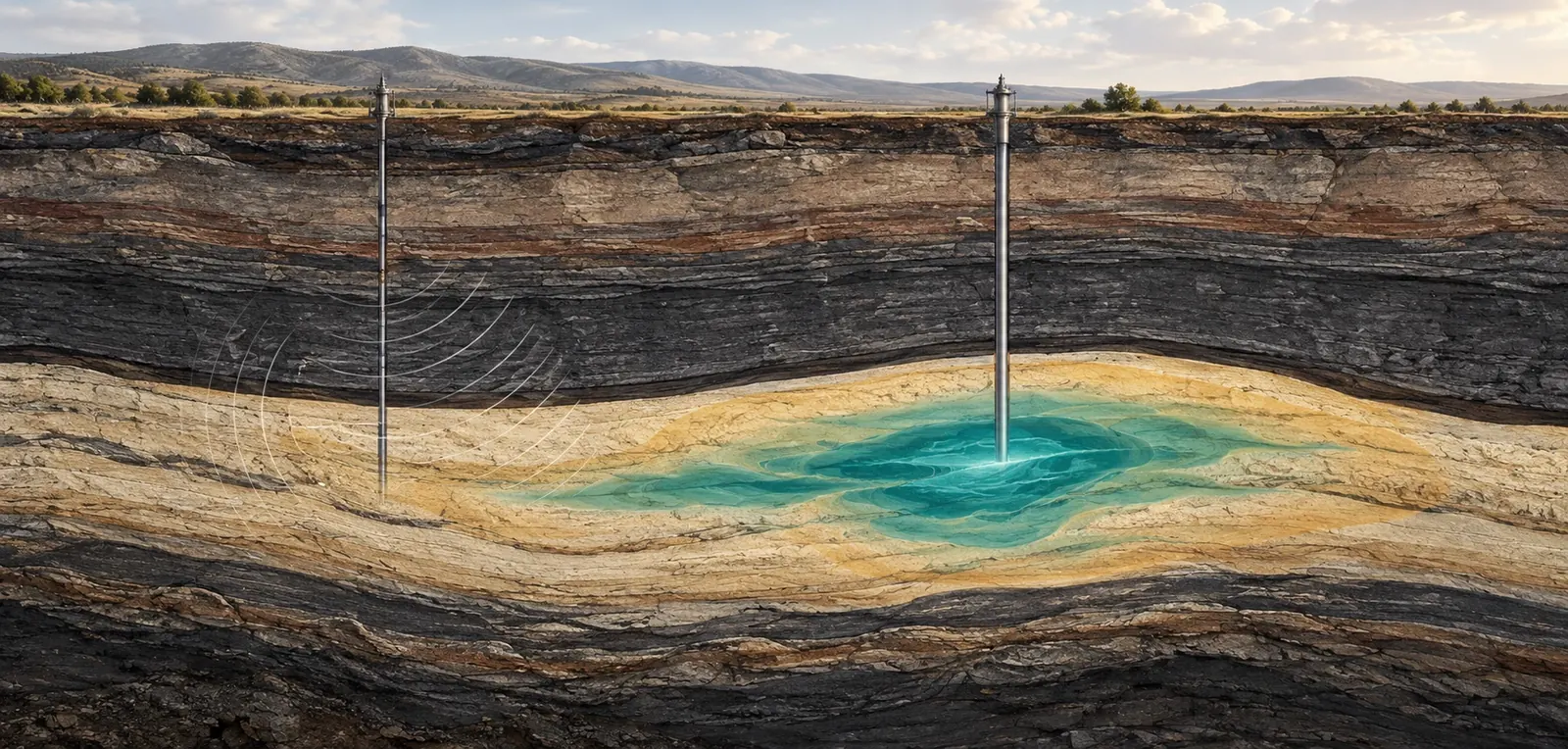
Geological storage monitoring turns echoes, pressure readings and surface motion into an account of what is happening underground. The difficult part is knowing which explanations those measurements can actually distinguish.
A computer can produce a beautiful underground plume before an instrument has measured anything. Give a simulator a geological structure, injection schedule and set of rock properties, and it will draw carbon dioxide spreading through the pore space. The animation may be physically plausible. It may also be wrong in precisely the place that matters: a thin barrier, an old well or the route toward a boundary of the storage complex.
That gap between a plausible picture and a supported interpretation is the central problem of geological storage monitoring. A February 11, 2025 preprint by Abhinav Prakash Gahlot, Rafael Orozco and Felix Herrmann proposed a three-dimensional digital shadow that updates possible plume states using time-lapse seismic observations. Its demonstration used a synthetic geological model and simulated observations. The research therefore tests an inference method under constructed conditions; it does not document successful containment at an operating storage site. Its usefulness as a starting point is that uncertainty is represented inside the calculation rather than appended to the final illustration. Gahlot and colleagues, version 1.
Imagine reviewing two reports about the same underground operation. One contains an attractive colored volume captioned as the stored carbon dioxide. The other contains several candidate volumes, the observations used to discriminate among them, the properties that remain poorly constrained and a forecast against which the next survey can be judged. The second report may look less decisive. It gives the reader far more ways to determine whether the project is learning.
This article follows that distinction through the measurement chain. It concentrates on subsurface observation, pressure and interpretation rather than the economics of carbon removal. The hypothetical examples are deliberately simplified and are not operating instructions or representations of a real storage site. Their purpose is to expose errors that a polished map can conceal: treating a pressure footprint as a gas footprint, treating an acoustic response as a mass measurement, or treating agreement with yesterday's data as proof of tomorrow's behavior.
Two footprints occupy the same rock
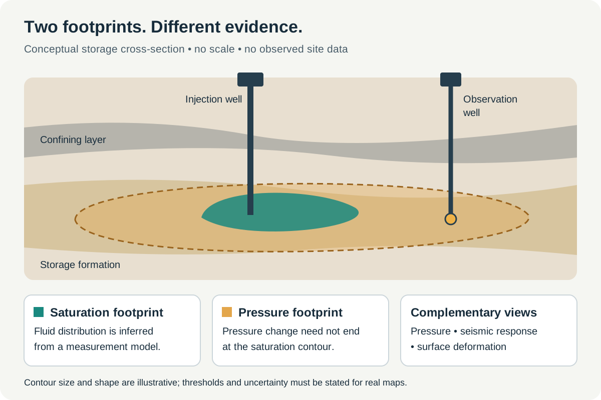
Conceptual illustration, not a measured site map. A saturation footprint and a pressure-change footprint represent different quantities; their thresholds and uncertainty must be specified for an actual project.
The phrase “the plume” can become dangerously elastic. It might refer to a region containing a separate carbon dioxide phase, a region where dissolved carbon has changed, or the much wider zone in which pressure has been affected. A report that switches among these meanings can seem internally consistent while describing different physical quantities.
The US Environmental Protection Agency's Class VI framework distinguishes the injected carbon dioxide plume from the associated pressure front in determining the area of review. Its regulatory purpose includes protecting underground sources of drinking water, and its monitoring expectations encompass both injected fluid and displaced formation fluids. A Class VI description should therefore not be presented as a certificate of net climate benefit; it addresses a particular underground-injection problem. EPA's Class VI overview.
A useful conceptual picture has two transparent overlays. The first marks where a chosen saturation threshold has been exceeded. Saturation is the fraction of available pore space occupied by a fluid phase, not the fraction of the total rock volume. The second marks where a chosen pressure change has been exceeded. The overlays need separate legends. Neither threshold should be hidden in the rendering software.
Consider a fictional map in which the saturation contour encloses a circle of radius one kilometre while a pressure-change contour reaches three kilometres. Those are invented dimensions, chosen only to make the arithmetic visible. The first circle covers approximately 3.14 square kilometres; the second covers about 28.27. The area ratio is nine, even though the radius ratio is three. A well outside the displayed saturation contour can consequently remain relevant to the pressure investigation. Nothing about this example establishes an actual ninefold ratio at any operating project.
Threshold choice changes the apparent boundary. If the pressure contour is defined at a smaller change, it may enclose a larger area. If the saturation image excludes weak responses, it may omit a dilute or unresolved extension. A clean edge in a figure is often the edge of a definition, not a physical wall.
For a reader, the practical question is: what quantity does this boundary represent, at what threshold, at what date, and with what uncertainty? For the analyst, the next question is whether a conclusion changes when that threshold is varied within a defensible range. If the location of a supposedly irrelevant well moves from outside to inside the area under a modest plotting change, the report needs to explain the sensitivity rather than select the more convenient image.
An echo is an observation, not a sample of gas
Time-lapse seismic work compares measurements acquired at different times. The interpretation depends on how changes in the underground state affect the recorded wavefield. The data must pass through acquisition, processing, imaging and a rock-physics relationship before they become a statement about fluid distribution. Each stage can introduce assumptions that are invisible in the final colored section.
Chadwick and colleagues' 2010 analysis of Sleipner examined how repeated seismic surveys could constrain the distribution of injected carbon dioxide in a favorable geological setting. The work treated thin-layer effects and the relationship between seismic response and plume geometry rather than assuming every bright reflection was a direct thickness measurement. Its importance is methodological as well as historical: a strong signal can still require a model to interpret what produced it. Quantitative analysis of time-lapse seismic monitoring at Sleipner.
An original thought experiment illustrates the distinction. Suppose a monitoring image contains a bright band that is one pixel thick. The image does not by itself establish that the physical layer is one pixel thick. Several thinner arrangements may produce responses that merge at the available bandwidth and sampling. Enlarging the image adds display pixels, not new information about the rock.
The same caution applies when a later image looks sharper. It may reflect a better acquisition, a different processing method or a more restrictive prior, as well as a real change underground. Comparing a blurry baseline with a sharpened repeat survey can create an apparent migration pattern that is partly a change in the representation. A defensible comparison keeps track of what changed in the measurement and what changed in the processing.
This does not make seismic monitoring futile. It makes the measurement model part of the evidence. A useful publication shows the observed difference alongside the predicted difference from the proposed underground state. It also displays the remaining mismatch at a scale where it can be inspected. The relevant test is not whether the proposed plume looks geologically reasonable. It is whether it accounts for the measurements more convincingly than competing plausible plumes.
One editorial test is surprisingly revealing: remove the color scale and ask the author to describe the actual recorded quantity. If the answer jumps immediately to tonnes, saturation or a leak rate, at least one inference step has been skipped in the explanation. Restoring those steps makes both the capability and the limitations of the method easier to understand.
How one volume can imply several masses
Mass estimation exposes the consequences of confusing a model parameter with a measurement. In a deliberately simplified uniform region, the mass of a separate carbon dioxide phase can be written as bulk volume multiplied by porosity, saturation and fluid density. This is a bookkeeping identity for the toy model, not a method for estimating an actual field inventory from a single seismic image. Dissolved material and spatial variability would require additional treatment.
Take an invented bulk volume of one million cubic metres, porosity of 0.20, saturation of 0.30 and density of 600 kilograms per cubic metre. The result is 36 million kilograms, or 36,000 tonnes. Now hold the bulk volume and density fixed while changing porosity to 0.15 and saturation to 0.40. The result is still 36,000 tonnes. Different internal descriptions produce the same mass because the porosity-saturation product is unchanged.
Reverse the question. If the image constrains only the apparent outer volume, it does not select between those descriptions. If the injected mass is well measured independently, that constraint can reject some combinations, but it still may not identify each parameter separately. A mass balance narrows the possibilities without turning every uncertain property into a known one.
The multiplication also reveals why percentage errors cannot be waved away. In the toy calculation, increasing porosity by ten percent while decreasing saturation by ten percent produces a product of 1.10 times 0.90, or 0.99 of the original value. The changes almost cancel. Increasing both by ten percent produces 1.21 of the original. Correlation among uncertain parameters matters. Listing four separate error bars without explaining their joint behavior can misrepresent the uncertainty in the quantity ultimately reported.
Romero, Luiken and Ravasi's 2023 preprint on joint inversion and segmentation of the Sleipner seismic dataset explicitly addresses limitations of band-limited seismic inversion and the use of additional structure in reconstructing plume-related changes. The accessible abstract supports that bounded methodological description; it is not used here as evidence for a particular recovered mass. Seeing through the CO₂ plume.
The implication for a storage report is concrete. Reported mass, mapped area and interpreted saturation should not be presented as three independent confirmations if one was calculated from the other two using the same assumptions. Readers need to know which quantities were independently observed, which were imposed as constraints and which were inferred. Otherwise an algebraic relationship can masquerade as a three-way agreement among instruments.
Pressure is both information and an operational constraint
A pressure history can be informative even when it is visually unremarkable. Its value comes from its relationship to injection history, well location and the alternatives a model predicts. A steadily rising trace means little without those reference points. A small departure at the right place and time may be more discriminating than a large change near the injection well.
EPA's March 2013 testing and monitoring guidance separates several tasks, including characterization of injected material, mechanical integrity, pressure monitoring, groundwater monitoring and tracking the plume and pressure front. That separation is useful beyond the regulatory setting: no single stream of observations answers all those questions. The guidance is a technical planning document, not evidence that any particular project has met its requirements. Class VI Well Testing and Monitoring Guidance.
Consider two fictional reservoir models. Both reproduce the pressure at an injection well during a period of steady operation. Model A communicates readily with the surrounding formation. Model B contains a restrictive boundary but compensates by using a different local permeability. At the injection well, the two explanations may be difficult to distinguish. At a more distant observation point, their predicted responses can separate.
The best next measurement is therefore not necessarily another instrument beside the existing one. It is a measurement whose expected behavior differs between the surviving explanations. A second instrument near the first can still be valuable for detecting sensor faults, but redundancy against instrument failure and information about geological uncertainty are different benefits. A monitoring plan should say which benefit it is purchasing.
An intentional change in operation can sometimes make a system easier to interpret, but a general-interest article cannot prescribe such interventions for a real site. The safe analytical point is narrower: observations need to be evaluated against the actual time history of the input. A pressure change following an altered injection rate is not equivalent to the same change under constant conditions. Leaving the input history out of a chart removes information needed to understand the output.
Likewise, a pressure reading is incomplete without its reference and measurement location. A surface value, a downhole measurement and a calculated formation pressure should not silently replace one another in a time series. A transition between sensors can create a step that looks like an underground event. Preserving calibration and configuration records is part of interpreting the physics, not merely administrative housekeeping.
A successful history match can hide the wrong geology
A model is history-matched when its adjustable description has been made consistent with past observations to a specified degree. That is useful, but the phrase can conceal a large family of solutions. If different geological arrangements fit the same record, reporting only the most visually appealing member discards information that should affect the forecast.
Chadwick and Noy's 2010 Sleipner study compared flow simulations with time-lapse seismic observations and examined the role of structural information in matching plume behavior. It provides a field-based example of a basic difficulty: small details in the geological description can matter for migration, while the available observations may not constrain them uniquely. History-matching flow simulations and time-lapse seismic data.
Imagine a hypothetical storage layer with two possible routes around a structural high. Past measurements show the plume approaching the fork but not yet passing it. Two models match every survey so far. In one, the left route is slightly easier; in the other, the right route is. Their historical agreement is genuine, yet their next forecasts differ sharply. Averaging the two predicted outlines may draw a broad central lobe where neither model expects the material to travel.
That average is mathematically permissible and operationally misleading if it is interpreted as the single most likely pathway. A better display preserves the alternatives or maps the probability of occupancy at each location. Even then, the probability depends on the model family and its weights. It does not cover geological possibilities that the analyst never allowed into the family.
This is why a forecast test should be specified before the new survey is used to tune the model. If the same observation is first used to revise a prediction and then cited as proof that the prediction was accurate, the test has become circular. The useful comparison is the archived forecast against the later measurement, followed by a documented explanation of the revision.
The goal is not to punish a model for being imperfect. Every useful model simplifies. The goal is to discover where its simplifications matter. A model that fails in a documented and interpretable way may be more valuable than one whose parameters are repeatedly adjusted without preserving the record of what it previously expected.
Surface movement adds another view, with another inverse problem
At In Salah, satellite radar observations were used to investigate surface deformation associated with underground injection. Vasco and colleagues' 2010 paper inferred subsurface behavior through an elastic model and considered both reservoir volume change and a fault or fracture-related feature. The interpretation depended on the assumed Earth model. Surface displacement was informative, but it did not directly identify the composition of every moving fluid underground. Satellite-based measurements of surface deformation.
This is an important example of complementary evidence. A seismic response, a pressure record and a surface-motion pattern do not have identical sensitivities. Combining them can reduce ambiguity. It can also import several different kinds of model error into one apparently unified answer.
To see the distinction, consider a fictional linear problem with two unknowns, x and y. Instrument A measures x plus y. Instrument B measures two times x plus two times y. The second measurement may be more precise, but it points along the same direction in parameter space. If A reads ten and B reads twenty, the pair still permits x equal to four and y equal to six, or x equal to seven and y equal to three.
Now replace B with an instrument measuring x minus y. If that reading is two while A remains ten, the equations give x equal to six and y equal to four. The second type of measurement has broken the ambiguity because it responds differently to the unknowns. Real geophysical problems are nonlinear and much larger, but this elementary example captures why diversity of sensitivity can matter more than the number of instruments.
It also shows why two interpretations are not independent merely because they were made by different software packages. If both begin with the same uncertain geological geometry and the same restrictive assumptions, their agreement may partly reflect a shared input. Independence should be described in terms of evidence and assumptions, not organizational separation alone.
A 2013 comparative study by Verdon and colleagues examined geomechanical responses at Sleipner, Weyburn and In Salah. The accessible abstract and figure descriptions support the conclusion that injection-induced behavior must be evaluated in its site-specific pressure and geological setting. They do not justify transferring a monitoring threshold or a safe operating pressure from one reservoir to another. Comparison of geomechanical deformation at three storage projects.
The timing of a change can be more valuable than another quiet survey
A September 4, 2026 preprint by Elling Svee and colleagues used a reduced model of migration through layered rock, with effective parameters for passage across thin barriers. It combined a Sleipner application with synthetic tests. The authors found that the information supplied by monitoring depended on which migration events the observations captured, rather than simply the length of the observation period. This remains preprint evidence, and the reduced model is not a complete description of every process near an injection well. Bayesian inversion of multilayer migration.
The distinction suggests a useful question for a fictional monitoring budget: what would the next survey teach that the last one did not? Repeating the same measurement at a fixed interval has operational advantages. It produces a regular record and may reveal changes nobody anticipated. But regularity alone does not guarantee that each new measurement will discriminate among the remaining geological explanations.
Imagine three candidate models that predict almost identical plume outlines for the next six months, then diverge after a layer-to-layer migration event. A survey before that divergence may provide a valuable check on instrument stability while adding little information about the disputed barrier. A later survey might be more informative about that parameter. Conversely, waiting too long could miss the timing of the transition, leaving only an end state that several models can reproduce.
This is an argument for matching observation design to the question, not for automatically reducing survey frequency. Safety-related surveillance and parameter estimation have different objectives. A measurement can have little value for refining a geological parameter and still be essential for detecting an unacceptable change. Combining those objectives into a single “information score” can hide a judgment about which failures matter.
A well-designed plan should therefore contain at least two explanations of its timing. One addresses the detection task: what departure needs to be noticed, and how much delay is acceptable? The other addresses the learning task: which competing predictions can this observation separate? The answers may favor different instruments or different sampling intervals.
The record should preserve quiet periods as well as unusual ones. If only surveys associated with an interesting result are displayed, the reader loses the denominator needed to evaluate performance. The same applies to unsuccessful methods. An instrument that repeatedly failed under the site's conditions is part of the evidence about feasible monitoring, even if it contributes no attractive figure to the final report.
How a model becomes overconfident
A probability map can look more sophisticated than a single deterministic outline while retaining the same basic blind spot. Its uncertainty represents variation within the assumptions used to generate it. If those assumptions exclude an important geological configuration, the map can be precise about the wrong set of possibilities.
Here is an original numerical example. Suppose a monitoring team considers twenty equally weighted candidate models. A new observation is much more consistent with five of them than with the other fifteen. For illustration, give each of the five a relative likelihood of four and each of the remaining models a likelihood of one. The first group then receives a combined weight of twenty out of thirty-five, about 57 percent. The observation has shifted the balance of evidence, but it has not made the favored group certain.
Now suppose the five models all share an untested assumption about a barrier. Adding more versions of those same five models does not independently validate that assumption. If each is duplicated ten times while the alternatives are left alone, an uncritical count of ensemble members will make the favored family appear overwhelmingly common. The result would reflect how the ensemble was constructed, not new underground evidence.
This is why an uncertainty display needs an explanation of weighting and sampling. A hundred realizations are not automatically a hundred independent geological hypotheses. Nor does a narrow distribution establish that important alternatives were tested. The reader should be able to ask whether the spread comes from sensor noise, uncertain parameters, different geological structures or different physical models.
A useful adversarial exercise is to hold out a class of plausible scenarios during development and then see whether the inference system recognizes unfamiliar observations. An honest result might be a warning that the new measurement does not resemble the training or calibration conditions. A less trustworthy system always returns a confident plume, even when the data no longer fit its world.
For communication, the distinction can be made without a lecture on statistical machinery. Separate the statement “these observations favor this interpretation among the tested alternatives” from the stronger statement “these observations exclude all important alternatives.” The first can be well supported while the second remains unjustified. An uncertainty-aware workflow earns its name by keeping that boundary visible when new information arrives.
Choosing measurements that can change a decision
Nilsen and colleagues' 2017 study used flow-model sensitivities and experimental-design methods to examine which measurements were informative about a Sleipner model. It also considered how different types of observations could provide complementary constraints. The paper's modeled information gains depend on the assumed physical situation and observation errors; they should not be converted into a universal prescription for fewer surveys. Using flow models with sensitivities to study monitoring programs.
The practical application is a disciplined comparison of candidate observations. In an original hypothetical example, a team is choosing between improving the precision of an existing sensor and adding a less precise sensor at a new location. The first option might halve the uncertainty in a quantity already well constrained. The second might distinguish two migration routes that imply different exposure of a legacy well. A ranking based only on instrument precision would miss the second option's decision value.
The comparison needs a declared decision. If the question is whether to investigate an unexpected pathway, the useful measurement is one that changes confidence about that pathway. If the question is whether a sensor has drifted, collocation with a reference may be more valuable. If the question is whether a regional model extrapolates beyond its calibration area, an observation away from the existing network may be essential.
Costs also need the right boundaries. Purchase price is only part of a monitoring system's burden. Access, repeatability, maintenance, data handling and the ability to preserve a comparable record can determine whether an initially impressive technique remains usable. These are design considerations, not a claim that a particular technology is cheaper at a particular site.
A proposed efficiency improvement should be tested against more than the model that suggested it. Removing an observation because the preferred model predicts little change there can make the network less capable of detecting that model's failure. One safeguard is to ask how the proposed network performs under credible alternatives, including scenarios in which the expected migration route is wrong.
This produces a useful distinction between optimization and resilience. Optimization makes a measurement program efficient for a specified set of conditions. Resilience preserves some ability to notice that those conditions do not apply. A program can be excellent at the first and weak at the second. The balance cannot be read from a single cost-per-survey number.
When the surface signal has several possible causes
An elevated carbon dioxide concentration near the surface is an observation that needs attribution. It does not automatically identify an underground storage source. Conversely, the absence of an anomaly in a limited sampling campaign cannot establish that no relevant change occurred anywhere or at any time.
A 2024 EGU conference abstract by Zhang and colleagues described seventeen years of soil-gas work at the Otway site and emphasized substantial year-to-year variability. The authors discussed combining different lines of analysis to investigate anomalies and favored risk-based monitoring with greater temporal resolution at selected locations. This is a conference abstract, not a full methods paper inspected here; its site-specific judgment about the usefulness of soil-gas monitoring should not be generalized into a universal rule. Otway soil-gas assurance-monitoring abstract.
The statistical problem can be illustrated without assuming any actual leak rate. Suppose one hundred independent tests are each set to flag a result with a five-percent false-alarm probability under a simplified no-change model. The expected number of flags is five. The probability of at least one flag is one minus 0.95 raised to the hundredth power, approximately 99.4 percent. These invented assumptions do not describe a real monitoring network, where observations may be correlated and thresholds more sophisticated. They show why “an anomaly was found” is incomplete without the testing context.
Nor does a multiple-testing explanation license dismissal. A flagged location can warrant investigation even when some false alarms are expected. The useful next step is to ask whether the pattern is coherent across time, space and independent measurements. A repeatable anomaly linked to an identifiable pathway is different evidence from an isolated exceedance produced by a single instrument on one visit.
A report should preserve both the initial flag and the subsequent reasoning. Reclassifying a signal after investigation is legitimate. Quietly deleting it from the record is not. The history matters because the same type of anomaly may recur, and because a future analyst may have better information about its source.
Attribution also needs a clear separation between environmental observation and engineering diagnosis. A measurement at the surface may establish that something unusual occurred there without identifying the route by which it arrived. A subsurface model may propose a route without proving that it supplied the measured material. The investigation becomes stronger when those statements are joined by evidence rather than by the convenience of a common narrative.
A monitoring record has to survive its own software
Long-lived storage creates a second kind of persistence problem: preserving the ability to interpret old measurements. A later analyst may need to compare a new survey with a baseline acquired using equipment and software that no longer exist. Keeping a final image alone is inadequate for that task.
Consider a fictional project that replaces its processing workflow after five years. The new software produces a small systematic shift in the mapped edge of the plume. If old and new images are compared without reprocessing a common dataset, the shift can look like migration. If both workflows are run on overlapping data, the team can estimate how much of the change is methodological. This is an original quality-control scenario, not a claim about a documented project's conduct.
The same logic applies to sensor replacement. An overlapping comparison can reveal an offset before the old device is removed. Where overlap is impossible, the uncertainty introduced by the transition needs to remain attached to the record. A continuous-looking line should not imply continuous measurement conditions when the underlying system changed.
A durable package should allow a technically competent reader to reconstruct the chain from observation to interpretation. That means preserving measurement coordinates and reference systems, acquisition configuration, relevant calibration information, processing versions, parameter choices and the relationship between observations and model outputs. Access permissions and proprietary constraints can complicate disclosure, but they do not remove the need for the operator and relevant reviewers to retain a coherent record.
The most valuable archived object may be a forecast that turned out to be wrong. It records what was believed before the next observation, which makes genuine predictive evaluation possible. If each model update overwrites its predecessor, the project retains only its current explanation of the past. That can be a useful engineering state, but it is a poor scientific memory.
For public communication, the record can be much smaller than the full technical archive. A dated sequence of predictions, observations, unresolved discrepancies and resulting changes can show whether monitoring is influencing decisions. This is more informative than repeatedly presenting a single confidence statement whose underlying basis changes without explanation.
A detection claim needs a specified challenge
The statement that a monitoring system can detect a change is incomplete unless the change has a size, location, duration and physical form. A method that detects a broad alteration in one layer may miss a smaller feature in another. A method that works well under one background condition may perform differently when the background changes. Detection capability belongs to a defined test, not to an instrument in the abstract.
A useful original test design starts with the unchanged observations and introduces a set of clearly labeled synthetic challenges. The analyst attempts to recover them without being told which records contain which challenge. The resulting table separates successful detections, missed challenges and false alarms. Its value depends on whether the simulated challenges resemble the departures that matter. Adding an unrealistically obvious signal only demonstrates that an obvious signal is detectable.
Suppose, purely hypothetically, that a method detects eighteen of twenty injected test signals of one specified type. The observed detection fraction is ninety percent for that small test set. It does not establish ninety-percent detection for every possible underground departure. Repeating the test across locations and background conditions may reveal a strong pattern: good performance near one survey line and poor performance elsewhere. Averaging those results into a single headline would erase the information needed to improve the network.
The challenge model itself needs scrutiny. If the same forward model generates the test signals and is used to recover them, the experiment may underestimate the consequences of model mismatch. A second set of challenges generated with different plausible assumptions can expose that weakness. The point is not to demand an impossible simulation of every future event. It is to make the domain of the detection claim explicit and to identify where the evidence is thin.
This approach also clarifies what happens after injection stops. The cessation of a controlled input does not automatically terminate the need to interpret the state already created. A hypothetical model might predict declining pressure while still allowing redistribution of the injected material. A report focused on only one quantity could therefore mistake a calmer pressure record for a complete description of subsequent behavior. The relevant questions and observation schedule should follow the evolving state, within the applicable site-specific requirements.
A closure argument needs a forecast over a stated horizon, evidence that the relevant measurements can test that forecast, and an account of remaining pathways and uncertainty. It should not rely on a countdown that becomes reassuring simply because time has passed. Conversely, every small adjustment to a contour is not evidence of failure. The same measurement and attribution discipline needed during injection remains necessary when the project is deciding what a quieter record means.
What an informative storage update would say
A strong update would begin with the underground question, not the instrument inventory. It would specify which aspects of plume movement and pressure were being tested, identify the observations obtained and distinguish measured quantities from inferred ones. It would then show where the observations agreed with the previously archived forecast and where they did not.
The update would make its blind spots concrete. It might say that a particular thin feature remains below the resolution of the available survey, that two migration pathways still fit the record, or that a sensor transition has widened uncertainty for one period. Those statements are more useful than an undifferentiated claim that uncertainty has been considered.
It would also explain what follows from the evidence. Some discrepancies might require a different geological model. Others might require an instrument investigation or additional observations. The account should distinguish a revised interpretation from a physical change in the underground system. A newly drawn contour can result from better knowledge of an existing state rather than a newly occurring event.
Finally, the update would state what future observation could challenge its conclusion. That is the feature that turns a reassuring picture into a testable account. Monitoring becomes scientifically persuasive when it creates opportunities to discover that the current explanation is incomplete, and when the project retains enough information to act on that discovery.
The underground plume will remain invisible to ordinary sight. Its behavior can nevertheless become increasingly constrained by measurements that respond to different properties, models that preserve credible alternatives and comparisons made before the answer is known. The aim is not an animation that never changes. It is an account of the subsurface that becomes harder to fool as the record grows.