
A precise isotope result can still permit several histories. Annual tree rings, reservoir models and explicit assumptions determine which calendar claims the evidence can support.
A tree ring can have a known place in a sequence and still complicate the history of an eruption. On February 12, 2026, Pınar Erdil and colleagues published new annual radiocarbon measurements relevant to the disputed timing of the Minoan eruption of Thera. Their comparison did not find compelling evidence for a rapid radiocarbon-production increase in the investigated period. Smaller differences among datasets remained, with several possible explanations rather than one established cause. This was a contribution to a difficult chronology, not an announcement that the eruption's calendar date had finally been settled. Erdil and colleagues
The distinction matters beyond one volcano. A radiocarbon measurement and a historical date are different kinds of information. The measurement describes carbon relative to a reference. The historical question asks when something happened. Connecting them requires a record of past carbon conditions and an account of how the sampled material relates to the event. Better measurements make that connection more demanding, not less important.
Imagine being handed a result with a narrow uncertainty and a request to place it beside a named ruler, a migration or a climatic transition. The temptation is to perform a subtraction and return a year. Yet the most informative answer may be two separated calendar intervals, a probability of being earlier than another event, or a statement that the available evidence cannot discriminate between competing sequences. Those are not evasions. They are different answers to different questions.
Radiocarbon's power lies partly in making those distinctions calculable. Its difficulties arise when a conventional age is treated as a calendar reading, a calibration curve as a perfect ruler, or an explicit chronological assumption as though it were another laboratory observation. Understanding the route between these objects reveals why scientific dating can be both extraordinarily precise and irreducibly conditional.
The number called an age
The reporting framework established by Minze Stuiver and Henry Polach in 1977 defined a conventional radiocarbon age using a specified reference, isotopic normalization and the historical half-life convention of 5,568 years. Its time origin is 1950: “before present” in this convention does not move forward with the year of publication. The resulting age is not already calibrated to calendar years. Keeping that convention stable allows measurements made at different times to remain comparable. Stuiver and Polach
A useful way to read the label is as a standardized coordinate, rather than a promise that a historical event occurred exactly that many ordinary years before the reference date. Changing the coordinate convention in the middle of an analysis would resemble changing the definition of a unit without changing the rest of the calculation. The apparent improvement could instead introduce an inconsistency.
The distinction becomes concrete in the age equation used by the National Ocean Sciences Accelerator Mass Spectrometry facility at Woods Hole. Its reporting documentation gives conventional age as minus 8,033 times the natural logarithm of the corrected fraction modern, often written Fm. The same documentation distinguishes raw isotope measurements, blank corrections and the final reported result. A process blank is material used to characterize contributions introduced through preparation and handling; measuring the sample is not the entire measurement system. NOSAMS reporting documentation
Here is an original arithmetic example, not a laboratory result. Insert a corrected fraction modern of one half into that logarithmic expression. Because the natural logarithm of one half is about minus 0.693, the conventional age is approximately 5,568 years. That agreement follows from the chosen convention. It does not establish a particular calendar year for a hypothetical artifact carrying that value.
Now change the fraction modern to one quarter. The calculation produces approximately 11,136 conventional years, twice the previous result. Halving a fraction adds an equal interval in this logarithmic coordinate; it does not subtract an equal number of years from a calendar without further information. Keeping the numerical example separate from a historical claim prevents a familiar equation from doing work that belongs to calibration.
Why subtraction cannot finish the job
Paula Reimer and colleagues' IntCal20 publication described a Northern Hemisphere calibration curve extending to fifty-five thousand calendar years before 1950. It combines independently dated evidence, with tree rings providing the fully atmospheric record back to roughly 13,900 calendar years before that reference. Older portions integrate other archives and their associated corrections and uncertainties. The paper is a documented 2020 curve release, used here to explain the method, not a claim that no subsequent research or revisions exist. Reimer and colleagues
Think of a calibration relationship as answering a forward question: if material formed at a proposed calendar time under the relevant carbon conditions, what radiocarbon result should be expected? Dating asks the reverse question. Given the measured result, which proposed calendar times remain plausible? A forward relationship can be well defined even when its reverse does not have one answer.
Consider a deliberately artificial calibration exercise. At calendar position A, the expected laboratory coordinate is one thousand units. At position B, fifty calendar years later, it is also one thousand units. At intermediate positions it differs. An observation near one thousand therefore need not select either A or B uniquely. Measuring it more precisely could sharpen both alternatives without removing either one.
This is not an actual stretch of IntCal20, and the units in the example are invented to isolate the geometry. The important operation is matching a result to a relationship, not subtracting the result from today's date. An instrument cannot distinguish two historical possibilities that the measurement model predicts will look the same, however many decimal places are printed on its report.
The analogy also explains why a single middle date can be misleading. If the evidence favors two separated periods and disfavors the years between them, their average could fall in the least plausible part of the answer. An average is a valid numerical summary of a distribution; it is not necessarily a representative historical possibility. A chronology should not acquire an unsupported central event merely because a table requires one number.
The curve is estimated too
The IntCal20 statistical-methods paper by Timothy Heaton and colleagues, published online on August 12, 2020, introduced a Bayesian spline approach with errors in variables. The method accommodates uncertainty in the calendar positions of some contributing observations as well as their radiocarbon measurements. It also addresses excess scatter and provides predictive uncertainty for calibration. The plotted curve is therefore an estimated relationship, not a collection of exact points joined by a line. Heaton and colleagues, curve construction
An original geometric example shows why the direction of uncertainty matters. Suppose a reference observation is placed ten calendar years too early on a fictional rising segment. If the expected radiocarbon coordinate changes by two units per calendar year, that horizontal displacement corresponds to twenty units vertically. Calling the vertical laboratory measurement precise would not repair the mistaken horizontal placement.
Conversely, suppose the horizontal placement is known exactly but the vertical measurement is uncertain. That is a different error structure. Combining observations from both situations requires more than treating every plotted point as an equally reliable dot. The model must preserve what is uncertain about each point rather than merely assigning a larger symbol to difficult evidence.
A graph can hide this distinction because both kinds of uncertainty ultimately affect the appearance of the fitted line. For a reader, the practical question is not whether the line looks smooth. It is whether the analysis carries the uncertainty relevant to the claim being made. The narrowness of a drawn line is a design choice unless the accompanying quantities explain what that line represents.
Nor is a more detailed curve automatically easier to invert. Extra structure may help distinguish some candidate dates while creating or revealing additional alternatives elsewhere. The gain is a better description of the reference evidence, not a guarantee that every unknown sample will yield a shorter calendar interval. Information can make an answer more complicated and more accurate at the same time.
Precision depends on where the sample lands
A local linear approximation offers a second original illustration. Imagine a fictional calibration segment rising by two radiocarbon years for each calendar year. A measurement uncertainty of twenty radiocarbon years would correspond, in that simplified neighborhood, to about ten calendar years. On another fictional segment rising by only one fifth of a radiocarbon year per calendar year, the same vertical uncertainty would correspond to about one hundred calendar years.
The calculation divides the vertical uncertainty by the magnitude of the local slope. It assumes a nearly straight segment, negligible curve uncertainty and no competing calendar solutions. Those assumptions are part of the example, not descriptions of a real period. At a turning point or across a broad plateau, the approximation breaks down and the full relationship must be considered.
This exercise explains why a laboratory improvement can have uneven chronological value. Reducing twenty units of uncertainty to ten would halve the local width in both invented examples, but the resulting calendar widths would still differ by a factor of ten. The same analytical achievement can answer one historical question decisively while leaving another unresolved.
There is a useful planning consequence. Before treating additional precision as the sole objective, ask what distinctions the proposed samples could make under plausible calibration shapes. Two hypotheses separated by centuries pose a different measurement problem from two hypotheses separated by a decade. A project can specify that desired distinction without pretending in advance that the available material will resolve it.
This is also a reason to state the question before choosing a summary. An inquiry into whether two activities overlapped is not identical to an inquiry into the midpoint of either activity. A narrow estimate for one event can coexist with substantial uncertainty about their ordering if the other event remains poorly constrained. Precision belongs to an estimated quantity, not to an entire historical narrative.
A hemisphere is part of the measurement model
Alan Hogg and colleagues' SHCal20 study presented a separate Southern Hemisphere calibration curve and discussed circumstances in which a mixture of hemispheric curves could be appropriate. Its evidence does not support treating the hemispheric difference as one timeless correction that can be subtracted from every sample. The relevant carbon environment and the study's geographic qualifications matter. Hogg and colleagues
This creates a distinction between identifying a sample's location and identifying the model appropriate to it. A coordinate on a map is useful evidence, but it does not by itself encode every process through which the sampled carbon entered the material. A transparent chronology records the chosen reference relationship and the justification for using it, instead of treating curve selection as an invisible software default.
Imagine two fictional analyses of the same measurement. One uses reference relationship North; another uses reference relationship South. If their resulting calendar intervals differ, that difference is not an independent laboratory disagreement. The observation has not changed. The assumed relationship between the observation and calendar time has changed.
The appropriate response is not to average the two published interval endpoints automatically. Such an average could lack any coherent model behind it. If a mixture is scientifically justified, the mixture needs to be represented at the appropriate level of the model, with its uncertainty. If the evidence instead identifies one reference as applicable, averaging in the other would discard that information.
For a public explanation, a short statement of the chosen curve can do considerable work. It makes the analysis reproducible and reveals a potential reason that apparently similar dates differ. Omitting it does the opposite: a result produced under a specific environmental assumption appears to be a direct and universal reading of time.
The ocean does not inherit the atmosphere's calendar unchanged
Marine20, developed by Heaton and colleagues in 2020, is a non-polar global-average marine calibration baseline rather than a direct substitute for an atmospheric curve. The study explicitly excludes unrestricted application in polar settings and treats regional variation through additional reservoir information. Its modeled ocean relationship propagates uncertainty in the atmospheric history and carbon-cycle parameters. A marine sample therefore cannot simply be assigned the terrestrial curve because both measurements are reported in radiocarbon years. Heaton and colleagues, Marine20
The inference problem is easiest to see with a fictional offset. Suppose an environmental process makes a sample's radiocarbon coordinate appear one hundred units older than the selected baseline would predict. If that offset is known exactly, the calculation can account for it. If it is only approximately known, correcting the central value does not remove the uncertainty in the correction.
Assume, solely for illustration, a measurement standard uncertainty of twenty units and an independent offset uncertainty of thirty. The combined standard uncertainty is the square root of twenty squared plus thirty squared, approximately thirty-six units. Reporting twenty after applying the offset would retain the precision of the measurement while silently discarding uncertainty introduced by the interpretation.
The word independent is essential in that arithmetic. If the two quantities share information, simple addition of variances may be inappropriate. Likewise, a correction inferred from a different time or setting does not become applicable merely because its number is available. A useful correction has both a value and a domain in which the evidence supports using it.
An environmental adjustment is thus not an inconvenience appended to an otherwise complete date. It helps define what the date means. Removing it from the explanation can make two results appear contradictory when they are actually based on different accounts of the carbon environment. Keeping it visible lets the disagreement be investigated at the correct level.
Mixtures must be mixed before the logarithm
A measurement on mixed carbon poses another mathematical trap. The conventional-age expression is logarithmic. Consequently, an arithmetic average of component ages is generally not the same as the age calculated from their mixed carbon fraction. The following example is entirely constructed and assumes equally weighted, comparably normalized carbon contributions, with no additional fractionation complications.
Let one component have fraction modern one half and another have fraction modern one quarter. Equal amounts of their carbon produce a mixed fraction modern of three eighths. Applying minus 8,033 times its natural logarithm gives about 7,879 conventional years. Averaging the two component ages instead gives about 8,352 years. The difference is approximately four hundred seventy-three years, despite the simplicity of the invented mixture.
Nothing in that calculation identifies an actual sample as contaminated or establishes the age of either component in calendar time. It demonstrates an order-of-operations problem. A physical mixture combines carbon contributions; the reported age is a subsequent mathematical transformation. Mixing the transformed numbers is a different operation.
The same issue appears if the mixture proportion is unknown. A single measured fraction can be consistent with many pairs of component fractions and proportions. More decimal places on the final mixture do not independently determine all of those unknowns. Additional information must constrain the components, their shares or both.
This is an example of a date that can be analytically precise yet historically ambiguous for reasons other than the shape of the calibration curve. The ambiguity begins before calibration, in the relationship between the measured material and its component carbon. A precise transformation of a mixture does not turn that mixture into a single coherent formation event.
For reporting, the useful distinction is between an observed fraction, a proposed mixing model and a calendar inference conditional on that model. Presenting all three as one undifferentiated “date” makes it difficult to tell which evidence would change the conclusion. Separating them identifies the missing information rather than hiding it inside an enlarged error bar.
Laboratories can test each other, not just their instruments
Lukas Wacker and colleagues' 2020 annual tree-ring intercomparison involved sixteen laboratories and three sets of twenty-one consecutive rings. It demonstrated strong capabilities for high-precision accelerator mass spectrometry while also finding that not every laboratory's results were always consistent with its stated uncertainties. That is evidence about the examined measurements and uncertainty estimates, not a current ranking of laboratories or a reason to dismiss the method. Wacker and colleagues
For an original thought experiment, imagine that two laboratories each measure the same fictional reference material ten times. Laboratory A obtains a tight cluster around one value; laboratory B obtains an equally tight cluster thirty units away. Each cluster demonstrates repeatability under its own conditions. The separation raises another question that within-laboratory repetition alone cannot answer.
Now suppose both laboratories repeat the exercise on three additional reference materials. If the separation persists with approximately the same sign and size, a shared offset becomes a candidate explanation. If the pattern changes with material or preparation, a simple constant offset may be insufficient. The design of the comparison determines which explanations can be distinguished.
There is no need to declare one laboratory right and the other wrong from this hypothetical pattern. The point is that independent replication can interrogate components of uncertainty that repeated measurements within a single setup may leave unchanged. The resulting investigation concerns the full route from material to result, not merely whether an instrument prints stable numbers.
A historical chronology also benefits from distinguishing repeated measurements of the same prepared material from independently prepared portions and entirely separate samples. All can be useful, but they probe different levels of the chain. Counting them together as interchangeable “dates” gives an inflated impression of how many independent opportunities the evidence had to disagree.
Nine measurements do not necessarily divide uncertainty by three
Suppose a fictional set of nine measurements shares one unknown calibration offset. Give every measurement an independent uncertainty of thirty units, and assign the shared offset an uncertainty of twenty. Averaging the independent components reduces their contribution to ten units. The shared component remains twenty. The uncertainty of the average is therefore the square root of ten squared plus twenty squared, about twenty-two units, not ten.
These values are original and the model is deliberately simple. Its purpose is to expose what repetition can and cannot remove. Nine observations of a common uncertain reference do not create nine independent references. The shared uncertainty is carried through the calculation rather than diluted by the number of observations attached to it.
There is a second, less intuitive consequence. If two estimated quantities share exactly the same additive offset, that offset cancels when one is subtracted from the other. Under the toy assumptions, their absolute positions may remain uncertain while their separation is better constrained. A real calibration relationship need not behave as one constant offset across a long interval, so that cancellation cannot be assumed indiscriminately.
This distinction is especially relevant to histories built from sequences. The evidence might establish that one event followed another by a relatively short interval while remaining less certain about the absolute calendar placement of both. A summary that reports only two independent-looking date ranges would conceal the relationship between them.
The reverse mistake is also possible: interpreting overlapping marginal intervals as proof that two events were simultaneous. Overlap describes the displayed individual estimates, not necessarily the joint probability of their difference. To answer a question about order, duration or separation, the analysis should calculate that quantity directly from the joint model rather than asking the reader to infer it from the shapes of two isolated bars.
Annual wood is not an instantaneous air sample
Bernd Kromer and colleagues studied earlywood and latewood cellulose from four tree species in a paper published in 2024. Their samples covered the atmospheric bomb-radiocarbon period, and the design included one tree per species. The measurements showed contributions from carbon stored in earlier years, with differences among the studied ring portions. This is evidence about the sampled trees and conditions, not a universal storage fraction for every member of those species. Kromer and colleagues
A simple invented filter illustrates the resulting interpretive issue without reproducing their observations. Suppose a recorded annual signal contains eighty percent of the current year's input and twenty percent of the previous year's input. Let the input be zero in every year except one, when it rises to ten arbitrary units. The recorded signal would be eight units in that year and two in the next.
The two-year response does not require a two-year input event. It follows from the stipulated storage rule. Conversely, observing a two-year response would not uniquely prove that particular rule; another process could generate a similar pattern. This is a forward demonstration of one possible effect, not a method for identifying a tree's actual carbon history from two numbers.
The example is useful because the annual label can otherwise be asked to mean too much. It may identify the ring's calendar position without implying that every carbon atom in the measured fraction entered the tree during that same calendar year. A temporal sample has a support: an interval or set of contributions over which it integrates information.
That support matters most when the question depends on a rapid change. A slowly varying input and a sharply changing input can respond differently to the same averaging process. Thus the fact that a sampling scheme works well for a broad background trend does not establish that it preserves every brief feature with the same amplitude or timing.
Averages can erase the very event being sought
Consider another original signal example. Ten annual measurements have values of zero except for one year with a value of ten. Their ten-year average is one. If the same total signal is spread evenly across all ten years, the average is still one. The average preserves the total under the stipulated equal weighting, but it cannot distinguish a brief excursion from a sustained modest elevation.
This is not a claim about any particular ancient cosmic event. It is the arithmetic of aggregation. Once the individual observations have been combined into one number, the within-block pattern is unavailable unless the original data or material retain it. A narrow error bar on the block average cannot restore information that the averaging operation discarded.
Unequal contributions make interpretation more complicated. If one ring supplies twice as much of the measured carbon as another, a simple arithmetic mean of their annual signals may not represent the bulk sample. The relevant weights belong to the measured contribution, not necessarily to the number of visible rings or the physical width of the cut sample.
The sampling decision therefore belongs in the chronology, not solely in a laboratory methods appendix. A research question about a century-long background shift may tolerate aggregation that would undermine a question about a one-year marker. Both projects can be technically competent while requiring different sample designs.
There is also a publication issue. A figure containing annual-looking points can imply a temporal resolution finer than the contributing material supports. Labels should reveal whether a point represents one ring, several pooled rings or a model estimate between observations. Otherwise the visual display supplies a precision that the underlying sample never possessed.
A pattern carries information that a single point cannot
Christopher Bronk Ramsey, Johannes van der Plicht and Bernhard Weninger's 2001 study examined methods for matching radiocarbon measurements with known age separations to the calibration relationship. Often called wiggle matching, this uses the pattern across a sequence, rather than independently placing every observation. Their comparison addressed both fit and uncertainty: finding a best alignment is not the same operation as establishing how uncertain that alignment remains. Bronk Ramsey and colleagues
Imagine three fictional samples known to be exactly ten calendar years apart. Each individual measurement might admit several placements. The combined sequence requires a placement at which all three predicted values agree with their observations while retaining the specified spacing. Alternatives that fit the first measurement but fail the second or third lose support.
The spacing is not an extra radiocarbon measurement. It is a different kind of evidence, and its reliability controls the force of the constraint. If the separation is only approximately known, the model should not silently treat it as exact. If one interval contains an unrecognized gap, an apparently sharp alignment can be sharp for the wrong reason.
A useful original analogy is a transparent strip bearing three marks. Sliding the strip along a reference pattern preserves the distances between the marks. Moving each mark independently would solve a different problem. Stretching the strip introduces another unknown. The analyst's task is to describe which of these operations the physical evidence actually permits.
This is why a sequence should retain identifiers and relationships, not merely a list of independently calibrated medians. Once the relational structure is removed, a later reader may be unable to reproduce the analysis or determine whether a changed assumption would alter it. The chronology resides partly in the arrangement of the evidence, not just in the values recorded for its individual pieces.
Priors can change an answer without changing a measurement
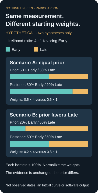
Original fictional calculation, not observed dates or a calibration curve. The same 4:1 likelihood ratio gives different posterior probabilities when the prior changes. Bars sum to one hundred percent; no actual chronology or software output is depicted.
Bronk Ramsey's 2009 methodological paper on Bayesian radiocarbon analysis describes a framework that combines measurements with constraints and groupings, and discusses testing chronological models with synthetic data. The accessible publisher abstract supports that general description; the full PDF was not available through the routes used for this article. The calculations below are original illustrations, not outputs reproduced from that paper or from an OxCal run. Bronk Ramsey, Bayesian analysis
Suppose a fictional dating problem has only two candidate hypotheses, Early and Late. Before considering a new measurement, assign each a probability of one half. Assume the observed measurement is four times as likely under Early as under Late. Updating those equal starting weights gives probabilities of eighty percent and twenty percent. The likelihood ratio supplies evidence in favor of Early, but it does not make Late impossible.
Now retain exactly the same measurement and likelihood ratio, while changing the prior weights to one fifth for Early and four fifths for Late. Multiplying the first by four and the second by one gives equal unnormalized weights. After normalization, the posterior is fifty percent for each. The measurement has not weakened; it has encountered a different starting distribution.
This toy comparison does not argue for either prior. It shows why a chronology should disclose where its additional information enters. If independent contextual evidence genuinely favors Late before the measurement, ignoring that evidence may be inappropriate. If the prior was chosen simply because Late was the desired answer, the calculation can conceal preference behind valid arithmetic.
The distinction between a model and a result can be tested by reporting both versions. Readers can see what the measurement contributes and how much the contextual assumption changes the conclusion. Such a comparison is more informative than announcing that a Bayesian model produced a precise date while withholding the assumptions that supplied much of the precision.
Ordering is not the same as spacing
Consider three fictional events, A, B and C. Evidence that A preceded B and B preceded C imposes an order. It does not establish that the intervals between them were equal, short or generated by a steady process. Adding any of those conditions would introduce more information than the order alone contains.
This difference can be made visible with simple candidate timelines. One places A at year zero, B at year one and C at year one hundred. Another places A at zero, B at ninety-nine and C at one hundred. Both obey the same order and span the same total duration. They tell very different stories about the timing of the middle event.
A model that distributes events uniformly within a period can favor certain arrangements over others. That may be a useful representation for a particular research problem, but it is not a neutral synonym for “some events occurred between these boundaries.” The assumed pattern of activity needs a rationale separate from the fact that the activity has a beginning and an end.
An effective sensitivity exercise therefore changes one meaningful assumption at a time. Keep the measurements fixed, then vary the allowed spacing, boundary behavior or classification of an uncertain sample. Observe which historical conclusions persist and which depend strongly on that choice. This does not require treating every imaginable scenario as equally plausible; it requires examining the plausible alternatives that could materially change the answer.
The strongest conclusion may be a limited one. Perhaps every reasonable model places A before a named transition, while the exact duration of the subsequent phase varies substantially. Reporting that stable relation can be more valuable than selecting the narrowest duration from the most restrictive model. Historical usefulness does not require presenting every output with the same degree of confidence.
An awkward date is a question, not an automatic deletion
In a separate 2009 paper, Bronk Ramsey developed treatments for outliers and offsets that distinguish measurement problems, contextual mismatches and shared deviations. The work includes approaches that downweight observations within a model rather than simply deleting inconvenient results. Its central relevance here is structural: an isolated discrepancy and a common offset across several observations are different possible explanations. Bronk Ramsey, outliers and offsets
Imagine a fictional group of six observations, five of which agree closely and one of which differs. Removing the sixth produces a tidy picture. But tidiness does not tell us whether that observation was mishandled, assigned to the wrong event, or correctly recorded evidence of a more complicated history. The choice among those explanations belongs to an investigation, not to the visual appeal of the remaining cluster.
Now imagine all six differ in the same direction from a proposed historical expectation. Treating each as an independent outlier could protect the expectation by construction. A shared environmental or modeling issue, or an incorrect expectation, would be competing possibilities. The pattern of disagreement matters as much as its magnitude.
A transparent report can preserve the observation, state the proposed explanation and show the effect of including or downweighting it. That does not force all evidence to carry equal weight. It makes the weighting inspectable and keeps the historical conclusion from depending on an invisible exclusion.
The phrase “consistent with the chronology” also needs care. If the chronology was built by selecting only observations that agreed with it, consistency supplies little independent confirmation. A more demanding test asks what evidence would have counted against the proposed ordering or date, and whether that evidence had a genuine opportunity to survive the analysis.
A reproducible chronology needs more than a date range
Imagine receiving two reports with identical final calendar intervals. One retains sample identifiers, measurement values, uncertainties, curve versions and model specifications. The other retains only a diagram and a sentence. At the moment of publication, their conclusions may look equally clear. When a reference curve, contextual interpretation or sample assignment changes, their usefulness diverges.
The first report permits a focused question: which input changed, and what happened when the same analysis was repeated? The second may require reconstruction from memory or secondary descriptions. Reproducibility is especially valuable when the change is small, because a small shift in an input can alter the balance between separated calendar alternatives without obviously changing the overall span.
An editorial presentation can preserve that structure without overwhelming every reader. The main narrative can state the historical question and the supported conclusion. A compact methods record can identify the measurement scale, calibration relationship, contextual constraints and relevant exclusions. A separate data record can retain the information required to recompute the result. Each layer serves a different reader, but all should describe the same analysis.
Version labels matter here in a mundane but powerful way. A result produced with one curve and one model is not reproducible merely because another researcher has the same software name. The inputs and model specification are part of the calculation. Recording them allows a later revision to be understood as a traceable change rather than an unexplained replacement date.
What the calendar answer should say
A defensible radiocarbon chronology does not have to apologize for uncertainty. It has to locate it. Some uncertainty belongs to the measurement, some to the reference relationship, some to the carbon environment, and some to the proposed relationship among events. These components can interact, but they are not interchangeable.
For a reader, the most revealing question is often simple: what additional evidence would distinguish the remaining possibilities? Another measurement of the same prepared material might address one concern. A different sample, a firmer sequence relation or a better environmental correction might address another. Repetition is valuable when it targets the uncertainty that actually limits the claim.
The calendar is therefore not hidden inside a carbon sample like a number waiting to be read. It emerges from a comparison between the sample, a reference history and a stated model of how the evidence fits together. When those connections are visible, a broad or divided answer can be scientifically stronger than a single confident year. The achievement is not merely assigning a date. It is showing why that date, and not the alternatives, deserves belief.