
Railway condition monitoring is learning to connect heat, vibration and impact to component health. The difficult test is not recognizing a damaged specimen; it is making reliable maintenance evidence from a changing railway.
The result that matters is the one that travels
A railway wheel does not need to be turning to produce an interesting diagnostic signal. In a preprint submitted on October 21, 2026, Aashish Shaju and colleagues examined the ultrasonic sound that decays after an impact on a stationary wheelset. Their study involved twenty-two wheelsets at two railroad facilities. A random forest transferred poorly between the datasets. A simpler detector based on two decay features did better; the more stringent wheelset-withheld evaluation correctly classified twenty-one of twenty-two wheelsets, with one healthy wheelset flagged. The authors call for additional independent data, including worn but serviceable wheels. This is promising stationary screening evidence, not a demonstrated accuracy rate for moving trains across a railway network. Shaju and colleagues, preprint
The contrast between the two classifiers is more revealing than the headline fraction. A method can recognize the examples available to its developers yet struggle with examples collected elsewhere. That is not a peculiarity of railways. But a railway makes the consequences unusually concrete: the object being classified has a maintenance history, carries loads, changes routes and eventually has to be inspected or repaired by someone who needs more than a score.
A useful monitor therefore has at least two jobs. It must produce a trustworthy observation, and the organization using it must understand what that observation justifies. Those jobs are related without being identical. A temperature is not a photograph of a bearing's interior. An impact force is not a direct measurement of every possible wheel defect. A model's confidence is not a certificate authorizing continued service.
This article follows the evidence from measurement to maintenance, rather than recommending operational thresholds or inspection intervals. All invented examples are explicitly hypothetical. They illustrate statistical and engineering reasoning; they are not instructions for deciding whether a real railway component is safe. The relevant decisions remain with qualified personnel working within applicable engineering and operating requirements.
Start by naming the object, not the algorithm
The phrase “railway fault detection” can conceal several different tasks. A wheel tread meets the rail. An axle connects and supports the rotating assembly. Bearings permit relative rotation while carrying loads. A defect affecting one of these elements can change signals measured elsewhere, but an observation associated with the assembly does not automatically identify the faulty element.
A diagnostic claim becomes clearer when written as a sentence with a specific subject and outcome. “This model distinguishes these damaged bearings from these reference bearings in these recordings” is narrower, and more informative, than “artificial intelligence detects train failures.” The narrower sentence exposes what still needs testing. It identifies the component, the comparison population and the evidence channel, instead of allowing the algorithm's name to do the explanatory work.
Consider a fictional maintenance database containing three columns: the component inspected, the reason for inspection and the final finding. A wheel can be referred because of an unusual impact, then receive a finding about its surface condition. A bearing can be referred because of unusual heat, then receive a finding after disassembly. If both records are reduced to a single label called “fault,” a learning system may be rewarded for predicting a mixture of conditions that require different interpretations.
This is a problem of definition before it is a problem of model capacity. Combining categories may be useful for a broad screening queue, but it makes the claim broader as well. A screen that identifies something worth examining need not be able to distinguish every underlying cause. Conversely, a model trained to identify a particular defect should not inherit credit for unrelated maintenance outcomes merely because they occur on the same vehicle.
A clear study description keeps the measurement unit and the decision unit visible. The sensor might generate thousands of short windows, the component might pass repeatedly, and the maintenance decision might occur once. Those are three different denominators. Reporting all three prevents a large number of recordings from masquerading as a large number of independently tested machines.
A hot reading is a measurement with a viewpoint
Constantine Tarawneh and colleagues reported a field comparison of wayside infrared readings and onboard bearing thermocouples in a 2018 conference study. Their instrumented train passed twenty-one hot-box detectors along a route of more than three hundred miles. The author abstract describes disagreement that depended on bearing class and measurement circumstances, including apparent temperature trends not present in the contact measurements. A related laboratory comparison reproduced similar tendencies. The accessible evidence is the university-hosted author abstract, not an independently inspected full proceedings paper. Its lesson concerns measurement comparability in that study, not the accuracy of every detector now operating. Tarawneh and colleagues
Two instruments can both be functioning as designed and still not be measuring the same effective quantity. Their viewing geometry, physical contact and response to changing conditions matter. Calling one reading “the temperature” can hide the question of which surface or location it represents. For this reason, a comparison needs a defined reference rather than a presumption that every sensor shares the same viewpoint.
Here is an original numerical example, unrelated to the reported temperatures. Suppose a stationary reference system reports a fictional value of sixty units, while an indirect monitor reports fifty-four. Calling the six-unit difference an error assumes that both readings estimate the same target under comparable conditions. If one estimates a different surface state, the comparison instead includes a physical difference as well as instrument error. Calibration cannot resolve a disagreement in the definition of the target.
The example also separates bias from variability. A monitor that is consistently six units low might be more predictable than one whose average error is zero but whose individual differences range widely. Neither description alone establishes fitness for a safety-related purpose. A useful report would show the distribution of paired differences, the conditions under which they were obtained and the uncertainty of the reference itself.
That last detail matters because the reference is part of the experiment. Treating it as infallible can make the candidate sensor look worse or better than the evidence supports. The purpose of comparison is to learn how the measurements relate, not simply to crown whichever device has been assigned the more authoritative name.
The track helps write the wheel's signal
Michele Maglio and colleagues combined instrumented wheelset measurements with numerical simulations in a paper first published online on June 7, 2021, and assigned to a 2022 journal issue. Their work related evolving wheel tread condition, rail roughness and contact circumstances to axle bending stresses. The measured and modeled responses showed why a stress signal cannot be interpreted solely as a property of the wheel. The study concerns a particular field campaign and a specified model of vertical interaction; it is not a universal conversion from vibration amplitude to remaining life. Maglio and colleagues, field measurements and simulations
The general inference is a familiar one in engineering: response belongs to a system. A wheel and a track interact, so a changing response can reflect either side of the contact, or a change in how the two meet. A monitor attached to the vehicle does not become independent of the infrastructure simply because its cable travels with the train.
A fictional paired comparison makes this visible. Imagine that a component's diagnostic score is twelve on route A and eighteen on route B. If the component has not changed between journeys, the six-point difference is evidence against interpreting the score as a pure measure of damage. It does not prove that route B is defective. It shows that the observed quantity includes context that must be accounted for before attributing change to the component.
Now suppose every component in the fleet receives a higher score on route B, while one component remains unusually high on both routes. The common shift and the persistent component-specific difference are distinct patterns. A model that keeps route context can ask about both. A model that erases context may call the common shift a fleetwide deterioration, or normalize away the unusual component along with it.
This is why a control group must be more than an arbitrary collection of normal-looking recordings. It should support the comparison actually being made. Matching on a convenient variable is not enough if another variable dominates the signal. The most convincing evidence shows which alternative explanations were examined, rather than merely demonstrating that a classifier can separate two folders of files.
Peak force and accumulated loading are not synonyms
A second Maglio study, published online on August 16, 2023, combined full-scale wheel-impact measurements with a model calibrated using measured three-dimensional tread geometry. It examined how operating conditions influence impact loads and used simulations to investigate effects on several running-gear components. The paper's numerical scenarios extend beyond the directly measured case and should be read as model-based assessments. Its important distinction is between observing a particular impact and interpreting the loading consequences of a damaged tread under varying conditions. Maglio and colleagues, impact loads and durability
A maximum compresses a history into one number. That may be appropriate for a particular screening rule, but it discards how often substantial loads occurred. Fatigue questions also depend on the sequence and distribution of loading, not merely on the largest value recorded during an arbitrary observation window. No single generic peak therefore supplies a complete history of material demand.
For an intentionally simplified arithmetic example, imagine two fictional histories expressed in dimensionless load units. History A contains one event of magnitude ten and ninety-nine events of magnitude one. History B contains one hundred events of magnitude four. A maximum-based ranking places A above B. A deliberately invented cumulative index that sums squared magnitudes gives A a total of one hundred ninety-nine and B a total of one thousand six hundred.
That invented index is not a fatigue law and cannot predict component life. Its value is logical: two summaries of the same observations can reverse the ranking because they answer different questions. It would be a mistake to adopt the index as a maintenance rule. It would also be a mistake to assume that a ranking based on the maximum answers every question about cumulative exposure.
The practical reporting implication is straightforward. When a study says one wheel is “worse,” the reader needs the quantity behind that comparison. Worse by peak impact, by estimated accumulated loading, by a confirmed defect or by a probability of future failure are materially different claims. A strong monitoring study connects its chosen signal to the specific outcome it intends to inform.
A laboratory crack is valuable without being an entire fleet
María Jesús Gómez and colleagues published a railway axle-monitoring experiment on June 24, 2020. They measured vibration at axleboxes on a full bogie installed on a rig, testing four axles with artificially introduced damage. Their method combined wavelet-derived vibration features with a support-vector classifier, and they examined the importance of training across different wheelsets. The result supports further investigation of condition monitoring between inspections. It does not constitute a naturally occurring service-failure sample, and its reported performance must remain attached to the rig, damage conditions and validation design. Gómez and colleagues
Controlled damage is useful because it makes the experimental question tractable. The researcher knows which specimen changed and can compare it with an earlier state. That control is an advantage, not an embarrassment. The limitation arises when the resulting dataset is treated as if it contains the full range of histories, materials and benign variation encountered in service.
An original thought experiment illustrates the distinction. Suppose a laboratory collects ten thousand windows from each of four specimens. A random split of individual windows could put recordings from every specimen into both training and test sets. The collection would contain forty thousand windows, while the test subset would contain no entirely unfamiliar specimen. A system could exploit persistent mounting or background characteristics while appearing to generalize impressively.
Holding out one whole specimen asks a harder question. Holding out a different test facility asks another. Neither strategy magically creates a representative fleet, but each removes a particular shortcut. The correct split depends on the intended claim: performance on another recording from a known assembly is not the same as performance on a newly encountered assembly.
This distinction also affects uncertainty. Repeated measurements of the same object are not equivalent to repeated independent objects. A narrow confidence interval calculated as though every window were independent can overstate the precision of the result. More recordings may improve characterization of the tested specimens while doing little to establish how the method behaves on a wider population.
Sound can carry evidence and the background together
Matthias Kreuzer and colleagues studied airborne sound from a commuter train equipped with healthy and damaged bearings, using two test trips to obtain realistic operating recordings. Their 2023 paper, available as a revised May 24 preprint accepted at ICPHM, used acoustic features and a neural classifier. It tested some bearing damage not included in training, while acknowledging the small number of fault types and the single scenario. The experiment involved intentionally installed damaged bearings and train test trips; it was not a random survey of naturally deteriorating bearings throughout a fleet. Kreuzer and colleagues
The attraction of sound is also its difficulty. A microphone records a mixture rather than a private channel from one component. A feature that helps identify the tested condition might also respond to a change in the surrounding soundscape. A successful field recording is therefore evidence that the signal can survive background complexity, not proof that every possible background has been handled.
Consider a fictional study in which all damaged specimens are recorded on rainy days and all healthy specimens on dry days. A classifier could achieve excellent accuracy by learning a weather signature. The example is deliberately exaggerated, but its logic applies to subtler differences in recording sessions, mounting, vehicle identity or processing history. The model does not know which distinction the investigator intended it to learn.
A useful check is to ask what information remains when the intended signal is absent. If the labels can still be predicted from filenames, session identifiers or other incidental metadata, the experiment contains a shortcut. Removing that shortcut from the input does not necessarily remove it from the waveform, where the recording environment may leave its own fingerprint.
This is not an argument against machine learning. It is an argument for experiments that make the desired interpretation difficult to fake accidentally. Performance on an unfamiliar component, a later campaign or a different recording environment gives a reader evidence about that interpretation. A large score without a clear account of what was unfamiliar leaves the central question unanswered.
Frequency needs a moving reference
A vibration frequency is a rate of repetition, not a label identifying the object responsible. The same recurring geometric feature can produce different repetition rates when the speed changes. Conversely, two different sources can produce the same rate under a particular set of conditions. This is a dimensional fact, and it helps explain why a feature extracted from a recording needs context before being assigned a mechanical interpretation.
Consider a wholly fictional, simplified wheel with a circumference of two metres, rolling without slip. At ten metres per second it makes five revolutions per second. At twenty metres per second it makes ten. A feature recurring once per revolution would therefore move from five to ten repetitions per second without any change in the feature itself. These numbers are teaching assumptions, not dimensions or diagnostic settings for an actual vehicle.
Now imagine a different source: a regular spatial pattern along an idealized track, with successive features two metres apart. At those same speeds, the encounter rates would also be five and ten per second. A single peak in a frequency representation would not distinguish the wheel-fixed source from the track-fixed source in this deliberately constructed example. The ambiguity follows from the chosen geometry, not from a defective algorithm.
Additional comparisons could make the hypotheses distinguishable in principle. A wheel-fixed pattern travels with the wheel, whereas a track-fixed pattern belongs to a location. But that distinction requires records that preserve component and location context. A frequency plot with those identifiers discarded cannot recover them simply by being analyzed more elaborately. The example concerns interpretation of evidence, not a procedure for testing running equipment.
It also explains why normalization is a scientific choice. Expressing a repetition rate relative to rotation may clarify a wheel-related pattern while changing how a location-related pattern appears. Expressing observations by distance rather than time answers another question. Neither transformation manufactures information about the source; each reorganizes the information already present under an assumption about what should remain comparable.
A well-described monitoring study therefore tells the reader which quantities were made comparable and why. Otherwise, an apparent shift in a diagnostic feature could be a change in the component, a change in motion or an artifact of the representation. Reporting the coordinate system is not mathematical decoration. It is part of stating what the measurement means.
A simulation knows its own assumptions
Afonso Lourenço and colleagues submitted a continual-learning study on February 18, 2026, combining vibration representations with information about axle passage and strain. The work examines adaptation across changing operating domains. Its quantitative experiments are based on simulated wheel–rail scenarios, including variations in vehicle, load, speed and track conditions. The paper is valuable as an investigation of model behavior under controlled changes, not as evidence of an already validated network-wide monitoring deployment. Reading the simulation section is essential to interpreting the word “experiments” in its performance claims. Lourenço and colleagues, preprint
A simulation offers something a field study rarely can: the ability to vary one assumption while holding others fixed. That makes it useful for discovering where a method depends on its inputs. But a simulated dataset inherits the simulator's representation of the world. An algorithm can become exceptionally good at detecting the patterns the simulator knows how to generate while remaining untested against patterns it omits.
Imagine an original fictional benchmark with three operating regimes called A, B and C. A model is trained on A, adapted to B and then evaluated again on A. If performance improves on B while collapsing on A, the update has traded old competence for new competence. Reporting only the new-regime score would hide that trade. Testing on C asks a different question about a regime not previously encountered.
Continual learning makes version history part of the scientific object. A prediction depends not only on the current measurement but also on which data the model has already absorbed. Reproducing the result therefore requires the order of updates, not merely the final architecture. A model that changes during evaluation can otherwise be credited with knowledge that would not have been available at the time of a real prediction.
For readers, the most useful distinction is between adaptation demonstrated within an experimental world and adaptation demonstrated after a real-world change. Both can be worthwhile. They are not interchangeable evidence, and neither automatically justifies allowing an operational model to redefine normality without a controlled evaluation process.
Detection probability belongs to an inspection system
Michele Carboni and colleagues' 2013 workshop paper examined ultrasonic detection in full-scale hollow axles using a set containing natural fatigue cracks and artificial defects. Their probability-of-detection analysis showed why equipment, calibration and inspection procedure must be considered together. A response obtained from a convenient reference defect cannot simply stand in for every real crack. The accessible original paper compares these influences; it is not used here to prescribe an inspection setup or an interval. Carboni and colleagues
Probability of detection describes how often a specified inspection system finds a specified class of defect under specified conditions. It is not the probability that a component is healthy after a negative result. The latter also depends on how common the relevant defect was before inspection and on what other evidence is available. Confusing these two probabilities can make a negative result seem more decisive than it is.
Take a purely hypothetical population of one thousand components. Suppose twenty contain a defined defect, and an imagined test detects eighteen of those twenty. Suppose it also flags forty-nine of the nine hundred eighty components without that defect. The test has ninety percent sensitivity in this invented population, but only eighteen of its sixty-seven positive results correspond to the defined defect. The arithmetic describes a screening problem, not any railway device's performance.
The unflagged group contains two defective components among nine hundred thirty-three negative results. That is a different conditional statement again. Changing the prevalence while keeping the test's assumed sensitivity and false-positive rate fixed changes the composition of the flagged and unflagged groups. The detector has not become a different instrument; the population to which its output is applied has changed.
These distinctions matter when moving from a deliberately enriched research collection to ordinary service. A study may include many damaged specimens because otherwise it would have too few informative examples. That is a sensible experimental choice, but its proportion of positive results should not be presented as the proportion a maintenance organization will encounter in a different population.
Three convincing removals do not measure every miss
Marco Barrera and colleagues described a pilot field test in a paper presented at the April 2022 Joint Rail Conference. Forty onboard devices monitored bearing-related vibration and temperature on railcars in a dedicated coal service. After two months, three wheelsets were selected for removal based on unusual monitored behavior, followed by inspection and laboratory evaluation. The paper reports preliminary field-to-laboratory comparisons. Such follow-up is valuable because it connects signals with physical examination, but selected removals alone cannot establish the number of defective components that a monitoring system failed to flag. Barrera and colleagues
The missing denominator is easy to overlook. If investigators examine only the flagged group, they can learn whether flags correspond to observable findings. They cannot directly estimate sensitivity, because sensitivity also requires knowing how many relevant defects existed in the unflagged group. A system that finds three genuine cases may still miss other cases; the three findings do not answer that question either way.
In an original fictional audit, suppose a screen flags fifty of five thousand components. Detailed examination confirms a target condition in thirty. The confirmed yield among examined positives is sixty percent. If no negative components are independently assessed, the total number with the condition remains unknown. Calling the system sixty percent sensitive would substitute one denominator for another.
There are also limits to the confirmation process itself. “No finding” can mean no defect was present, no defect was found by the chosen examination, or a condition had changed before examination. A defensible database records the inspection method and timing instead of treating every negative teardown report as a perfect historical reconstruction.
This is where maintenance records become scientific infrastructure. Linking the original signal, component identity, subsequent examination and final disposition supports learning from both apparent successes and disagreements. Without that link, the organization may accumulate an impressive archive of alarms while remaining unable to explain which alarms were useful, which were misleading and which relevant cases never produced an alarm at all.
A quiet stream can mean several different things
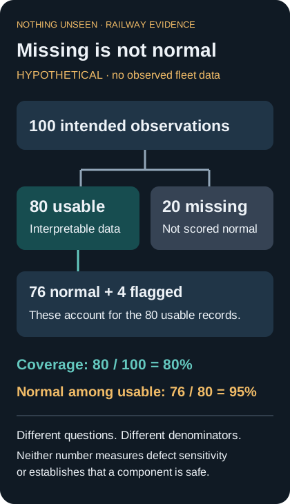
Fictional audit, not observed railway performance. Coverage and the fraction normal among usable observations answer different questions; missing observations are not normal findings. Neither quantity is detector sensitivity.
A monitoring system produces observations only when its measurement and recording chain succeeds. The absence of a reported anomaly is therefore not the same as evidence that all intended observations were normal. A component may not have been observed, a record may be incomplete, or the data may fail quality checks. Those possibilities belong in the evidence record rather than being silently absorbed into the normal category.
Consider an original fictional monthly summary covering one hundred intended component observations. Eighty are usable and twenty are missing. Of the usable observations, seventy-six meet the study's definition of normal and four are flagged. Reporting “ninety-six percent not flagged” by counting the twenty missing records as normal would be wrong. The observed normal fraction is seventy-six out of eighty; the coverage is eighty out of one hundred. Neither number substitutes for the other.
Missingness also has a pattern. If the unavailable observations all occur under conditions that are difficult to measure, the surviving records may overrepresent easy cases. A model evaluated only on those records could perform well precisely because its hardest intended operating conditions were removed before scoring. Reporting quality exclusions is therefore part of reporting performance, not a tedious appendix to it.
A useful evaluation can separate three outcomes: interpretable normal, interpretable abnormal and uninterpretable. That third category need not be a failure of honesty or sophistication. It may be the most accurate description of what the system knows. The scientific question is how often it occurs, under which conditions, and whether subsequent evidence resolves it.
The same separation applies to component identity. A beautifully measured signal linked to the wrong wheel is not a successful component-level observation. Identity errors can turn a useful detection into a misleading maintenance history. Evaluations should therefore consider the integrity of the complete record, not only the numerical quality of the waveform after it has been assigned to an object.
Early warning is a time-dependent claim
“Detected before failure” sounds decisive until the time reference is specified. A method may identify an abnormality shortly before a known event in a retrospective dataset, yet provide little evidence about how it would behave during the much longer preceding period. The result may still be scientifically useful. It simply answers a different question from whether a prospective monitoring system offers consistently usable notice.
An original hypothetical timeline clarifies the distinction. A component is observed on days one, five and nine, then examined on day ten. A retrospective analyst sees the examination result and chooses a feature that looks unusual on day nine. That analysis can identify a promising association. It cannot by itself show that an analyst on day five would have known which feature to trust or that the day-nine flag was specified in advance.
The relevant evaluation separates feature development from later testing. Once a rule has been defined, its behavior can be assessed over a new interval without changing the rule to suit the outcome. The report should include both the events it anticipated and the periods during which it generated concern without a corresponding confirmed finding. Otherwise the apparent warning time can be enlarged simply by selecting an earlier ambiguous fluctuation after the fact.
Lead time also needs an endpoint. Time before a workshop finding, time before a scheduled removal and time before a physical failure are not interchangeable. Maintenance often interrupts the natural history of a defect, which is desirable operationally but complicates claims about what would have happened without intervention. The avoided outcome is not directly observed merely because the component was removed.
This is an argument for carefully worded benefits, not for waiting for failures. A study can report earlier recognition of confirmed conditions, better targeting of examinations or improved scheduling evidence without claiming to have observed the failures that did not occur. Those narrower outcomes can be important achievements in their own right.
The maintenance action changes the dataset
Once a monitoring system influences maintenance, it also influences the evidence later used to evaluate that system. A high-scoring component may be removed promptly, while a low-scoring component remains in service. The two groups then receive different opportunities to develop a later outcome. A naive comparison can mistake this difference in treatment for a difference in underlying risk.
Imagine a fictional fleet in which every component receiving a high score is examined and, when appropriate, repaired. Months later, few high-scoring components have failed. It would be unreasonable to conclude that the original score was useless because those components did well. It would be equally unreasonable to claim that every removal prevented a failure. The intervention has changed the path being observed, so both conclusions require more evidence.
This problem can be addressed conceptually by recording the sequence of decisions. The data need to distinguish the state before examination, the examination finding, the work performed and the subsequent exposure. An aggregate field called “outcome: healthy” loses that history. A component healthy after repair is not equivalent to a component shown to have been healthy when it first triggered concern.
Comparisons also need a meaningful exposure measure. A component that travels little after an assessment has less opportunity to generate an observed service event than one that travels extensively. Calendar time alone may therefore be an incomplete denominator. The appropriate measure depends on the claim, and should be chosen before looking for the most flattering improvement.
These are evaluation principles, not a proposal to withhold maintenance for experimental convenience. Research can use independently justified inspections, established records and carefully bounded observational designs. The crucial point is that operational action and scientific observation are intertwined. A credible study makes that interaction explicit instead of pretending that a fleet continues unchanged while an algorithm watches from outside.
A network trend is not an isolated experiment
A Federal Railroad Administration report published in May 2022 examined detector deployment and historical derailment data. The report's project dates run from September 2008 through December 2012. Author Som P. Singh analyzed detector installation growth and vehicle-performance information alongside accident trends, reporting an association between expansion of several wayside technologies and fewer derailments. This is retrospective system-level evidence. It should not be converted into a randomized estimate of the benefit of one detector, or mistaken for a measurement of the railway network's condition in 2026. Singh, FRA technical report
System-level evidence matters because component experiments alone cannot show what happens after technology is embedded in an organization. But historical trends carry other changes with them. Traffic, equipment, maintenance practices and reporting can evolve during the same period. An association can be consistent with a beneficial contribution without identifying its exact share of the observed improvement.
An original hypothetical example shows why denominators matter even before causal attribution. Suppose a fictional network records twenty relevant events in one period and fifteen in a later period. The count falls by one quarter. If its exposure also falls by one quarter, the event rate per unit exposure is unchanged. If exposure rises, the rate improvement is larger than the count alone suggests. Neither calculation identifies the cause of the change.
A useful comparison therefore states the period, the population and the exposure basis. It also identifies whether the technology was introduced alone or alongside other changes. A study can be informative without eliminating every alternative explanation, provided it does not conceal those explanations behind a precise-looking percentage.
The evidence ladder is not a competition in which field databases automatically defeat laboratory work or vice versa. Each addresses a different uncertainty. Controlled tests can isolate mechanisms. Field campaigns can expose practical variability. Long-term records can show organizational patterns. The strongest maintenance argument connects these forms of evidence without pretending that any single one answers every question.
The useful output is an auditable history
Imagine opening a component's record after several months of monitoring. A useful history would let a reader reconstruct what was observed, when it was observed, which model interpreted it and what later examination found. It would distinguish a revised interpretation from the original prediction. It would preserve uncertainty rather than overwrite it with the final outcome. These are proposed qualities of an evidence record, not claims that every railway already maintains such a record.
Such a history also makes disagreements productive. Suppose a signal is repeatedly unusual but several examinations find no target condition. That pattern could indicate an unhelpful feature, an incomplete reference examination or a condition outside the original label definition. The record should support investigation of those possibilities. Deleting the observations as embarrassing false alarms would remove the information needed to understand the disagreement.
Likewise, a confirmed defect without an earlier flag should remain visible in the evaluation. The question is not how to make a dashboard appear clean, but how to learn the boundary of the system's competence. A method may work well for one class of condition and poorly for another. Stating that boundary is more useful than averaging the two into an undifferentiated success score.
For maintenance planning, the most valuable improvement may be better discrimination among cases that already deserve examination, rather than an entirely new claim of autonomous diagnosis. More consistent evidence can help explain why one component warrants closer attention, while the actual decision remains grounded in appropriate inspection and engineering judgment. That is a substantive contribution even without a dramatic promise to predict every failure.
The wheel at the beginning of this article produced a decaying sound, not an answer sheet. Its signal became evidence only through comparison, validation and limits on interpretation. Railway monitoring advances when those limits become sharper: when a stationary screen is not advertised as a fleet guarantee, when a field success includes its missed opportunities, and when a maintenance record can show how an observation changed what was learned. The goal is not a railway that never produces uncertainty. It is a railway whose evidence makes uncertainty harder to mistake for knowledge.