
Space laser communications can move extraordinary amounts of information. Turning a successful optical link into a dependable service requires accounting for everything that happens before, between and after the photons arrive.
A successful ending, and a different question
On September 18, 2025, NASA reported the completion of its Deep Space Optical Communications demonstration, carried aboard Psyche. The agency described a final, sixty-fifth pass from 218 million miles away and a cumulative receipt of 13.6 terabits. It also distinguished separate milestones: the maximum bitrate reached in December 2023 and the greatest transmission distance reached in December 2024. Those achievements did not occur at one interchangeable operating point. The dated account is evidence of a completed demonstration, not a declaration that every future spacecraft now has a continuously available optical connection. NASA's DSOC completion account
That distinction changes what a reader should ask of the next impressive number. How much information crossed the link while it was operating? How much reached the intended recipient before a deadline? How often did the opportunity to transmit exist? A record can answer the first question beautifully while leaving much of the other two unexplored.
An optical communications system is sometimes pictured as an extraordinarily long fiber with the glass removed. The image captures the use of light but conceals the difficulty of keeping the endpoints connected. A fiber supplies a continuous physical route. A space link must repeatedly establish a useful geometric and atmospheric route, identify the signal, maintain its alignment and deliver a recoverable sequence of information. The endpoint is moving even when the mission calendar calls the ground station a fixed facility.
The most revealing way to examine this technology is therefore not a league table of peak speeds. It is an accounting exercise across several different clocks: the time allowed for a contact, the time needed to find the other terminal, the time during which the atmosphere cooperates, and the time before the information loses its usefulness. Faster transmission can improve the outcome. It cannot make those clocks identical.
Consider the following journey through a fictional contact and a series of explicitly hypothetical design comparisons. None describes an actual mission's measured performance or supplies operational settings. Their purpose is to make the missing denominators visible, so that a reported result can be understood at the scale where it was actually demonstrated.
Start the ledger before the first bit
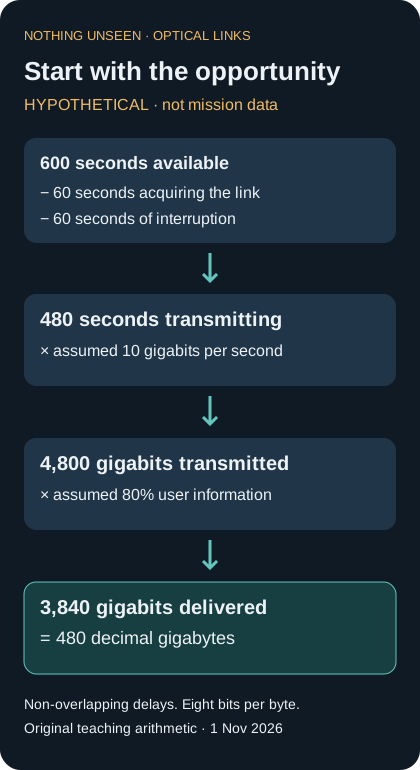
Fictional contact ledger, not measured mission performance. Delays are non-overlapping; the user-information fraction is assumed, not a universal optical-link efficiency. Decimal gigabytes use eight bits per byte.
Suppose a spacecraft has a ten-minute opportunity to communicate with a ground station. For this example, the advertised transmission rate is ten gigabits per second. Multiplying that rate by all six hundred seconds produces six thousand gigabits, or six terabits. That is a ceiling under the stipulated rate and window, not yet a delivery estimate.
Now reserve sixty seconds for acquisition and another sixty for a weather interruption. Assume those intervals do not overlap. Four hundred eighty seconds remain. At the same line rate they carry four thousand eight hundred gigabits. If only eighty percent of those transmitted bits are new user information after the particular fictional system's coding, framing and repetition costs, the delivered amount becomes three thousand eight hundred forty gigabits. Using eight bits per byte and decimal units, that is four hundred eighty gigabytes.
The calculation is deliberately simple. The phrase “eighty percent” is not a generic efficiency for optical communications. It is an assumed conversion factor within this example. An actual system might quote its rate after some of these costs have already been removed. Applying the factor a second time would understate delivery. Conversely, treating a raw optical modulation rate as verified scientific data could overstate it.
This is why a useful report names its counting boundary. Bits leaving a modem, correctly decoded frames at the receiver, unique files in ground storage and products delivered to a science team are different counters. Two teams can report different totals without either making an arithmetic error, because their counters sit at different places in the chain.
The fictional contact also shows why elapsed time needs a boundary. Was acquisition included in the reported five-minute interval? Were cloudy contacts omitted from the dataset? Does a daily average include days when no pass was scheduled? The same successful transmission can look excellent per active second and modest per calendar day. Neither description is inherently dishonest; a comparison becomes misleading when its denominator silently changes.
For a finite observation, there is another counter worth keeping: how much unique information remains onboard after the contact. A system that retransmits previously received material may consume the whole allotted window while barely reducing that backlog. The difference between traffic and new information becomes especially important when a mission has more observations waiting than one pass can carry.
Narrowness is an asset with a price
A narrow beam concentrates useful optical power, but concentration makes angular error consequential. Lorenzo Valentini and colleagues examined this tradeoff in a six-page analysis presented at Globecom 2021. Their models include errors at both terminals and distinguish a bound on angular error from a statistical outage calculation. The paper does not support the idea that increasing optical gain always improves the complete link: pointing losses must be included in the gain that actually remains useful. This is a modeling result under stated beam and error assumptions, not a measured failure rate for every spacecraft. Valentini and colleagues, pointing-loss analysis
An elementary geometric example puts angular language into physical units. At a hypothetical range of one million kilometres, an angular offset of one microradian corresponds to roughly one kilometre of transverse displacement, using the small-angle relation between angle, range and displacement. At ten million kilometres the same angular offset corresponds to ten kilometres. These are chosen round numbers, not a specification for any terminal or a claim about its beam footprint.
The comparison is useful because it separates two possible remedies. Reducing angular error changes where the beam lands. Widening the beam changes the area over which its energy is distributed. They can both affect whether a receiver collects enough light, but they are not the same improvement and need not have the same consequences elsewhere in a design.
Imagine two fictional designs tested under identical conditions. One produces twice as much received power when perfectly aligned but loses that advantage during frequent excursions. Another has a lower best-case level and a steadier time series. The choice cannot be made from the highest plotted point alone. The relevant question might be total recoverable information over a contact, or the chance of completing a particular file before the horizon ends the opportunity.
Even a summary of the angular errors can hide that distinction. An average signed error near zero might mean excellent alignment. It might instead mean errors on opposite sides of the target cancel numerically. A bound, a root-mean-square value and an outage fraction describe different features. They should not be treated as alternative spellings of “accuracy.” A report that states which one was measured gives the reader a way to connect the pointing claim to the communication claim.
Finding the link consumes the link's opportunity
Acquisition is not merely a ceremony before the real experiment begins. In a 2019 author manuscript, Muhammad Salman Bashir and Mohamed-Slim Alouini modeled acquisition with photon-counting detector arrays. Their analysis considered missed detections, false alarms and acquisition time under specified beam and noise assumptions, using analytical bounds and numerical comparisons. It is evidence about a mathematical search problem, not a timetable promising when an operational spacecraft will lock onto a station. Bashir and Alouini, signal acquisition
To see why the time matters, return to the fictional ten-minute contact. Suppose one design needs thirty seconds to acquire the signal and another needs ninety. Hold all other assumptions fixed. The difference is a full minute of potential transmission, not an inconsequential setup delay. At the stipulated ten-gigabit rate, the extra minute corresponds to six hundred gigabits of line-rate capacity before any other accounting adjustments.
However, simply choosing the design with the shortest average acquisition time may be premature. Imagine that the first design usually locks quickly but occasionally spends almost the entire window searching. The second consistently acquires after a moderate delay. If a contact must deliver a small, time-critical message, the long tail in the first design's acquisition distribution may matter more than its attractive mean.
A useful fictional test would therefore retain the unsuccessful attempts. Reporting only the time required on successful attempts answers a conditional question. A design that fails to acquire on many attempts could appear fast if those attempts disappear from the average. The report should distinguish “time to acquisition when acquisition occurred” from “probability of acquiring before the deadline.”
There is also an accounting consequence when a search is abandoned. The elapsed minutes do not return to the pass. Switching to another station, another mode or a later contact may be sensible, but that choice creates a new history of which data arrived when. An operator cannot evaluate the policy by pretending every unsuccessful attempt was costless.
This is an unusual feature of communications performance compared with a simple bench measurement. The apparatus must first create the conditions in which its headline performance can be exercised. Those conditions have their own uncertainty. The acquisition record belongs in the evidence, rather than being edited away to make the transmission graph begin at its most flattering moment.
The platform has its own motions
NASA's November 14, 2024 account of DSOC's pointing hardware describes a vibration-isolation platform developed by Controlled Dynamics Inc. Struts and actuators helped isolate the flight optical assembly from spacecraft motion; the account traces testing before its use on Psyche. It is an institutional account of a specific development path, not evidence that any commercial stabilizer can be substituted into any mission. The physical lesson is limited but important: knowing the intended direction and keeping an optical assembly on that direction are separate engineering tasks. NASA's precision-pointing account
A fictional acceptance test illustrates how an apparently minor change could matter. Suppose an optical assembly is first characterized on a quiet bench and later mounted beside equipment that switches between operating states. The combined system's pointing record must be examined in each relevant state. A successful quiet-bench result does not numerically determine the disturbance introduced by the neighboring equipment.
The sequence of events matters as much as the list of components. If a disturbance occurs during the first seconds of acquisition, it may delay the whole contact. If it occurs during an already established link, it may instead produce a brief interruption. If the same disturbance coincides with a change in atmospheric conditions, a single receive-power trace may not identify the cause. The problem is not solved by labeling every dip “weather.”
A disciplined fictional record would align the pointing telemetry, equipment-state changes and receiver observations to a common time reference. It would preserve enough timing detail to distinguish a sustained offset from a short excursion. This is a proposed diagnostic comparison, not a claim about unpublished telemetry from DSOC or another mission.
It would also state what the test did not exercise. A limited campaign cannot sample every possible combination of platform state, temperature and contact geometry. Rather than treating that fact as an embarrassment, an engineering account can use it to identify the next informative test. Confidence grows when a claim's range is explicit, not when a single successful trial is made to stand for an unlimited operating envelope.
A detected photon is not automatically a bit
Emma Wollman and colleagues' September 2024 author manuscript describes the detector system developed for DSOC's primary ground receiver. The work separates detection efficiency, background counts, timing jitter and count-rate behavior, and includes laboratory characterization as well as deployment context. Its definition of system detection efficiency begins at the cryostat's entrance window, not at the distant spacecraft. That boundary matters: an efficient detector does not recover photons that never entered the receiver. The paper also shows why one peak efficiency number cannot summarize every operating condition. Wollman and colleagues, detector-system study
Imagine, purely for arithmetic, that one hundred signal photons reach a chosen instrument boundary in a measurement interval. If eighty percent survive the next optical stage and seventy-five percent of those produce recorded events, the expected count associated with the signal is sixty. Multiplying the two fractions is appropriate only because they refer to consecutive stages of the same population in this hypothetical model.
It would be wrong to call that sixty-percent figure the fraction of all photons emitted by the spacecraft that were detected. The example starts much later in the journey. It would also be wrong to add the two losses as if each applied to the original hundred. Twenty photons are lost at the first stage; twenty of the remaining eighty are lost at the second.
Now suppose the instrument records additional events unrelated to the desired signal. Those events do not become useful information merely because the detector is sensitive enough to notice them. In a toy comparison, ten desired events mixed with one unwanted event create a different inference problem from ten desired events mixed with a hundred. The total recorded count rises in the second case, while the task of deciding which pattern was transmitted becomes harder.
Information can be carried by when a pulse arrives
A 2005 JPL report by Bruce Moision and Jon Hamkins develops serially concatenated pulse-position modulation with error-control coding. In pulse-position modulation, information is associated with the position of a pulse within a set of time slots. The report studies a particular coded scheme and decoder through analysis and simulation; its performance claims are not a guarantee for an arbitrary optical link. Coding, modulation and receiver interpretation belong together, rather than being interchangeable improvements to the laser's optical power. Moision and Hamkins, coded modulation
For an elementary teaching example, imagine four possible slots, labeled first, second, third and fourth. There are four possible pulse positions, so an agreed mapping can represent four alternatives, equivalent to two binary choices. Sixteen possible positions represent sixteen alternatives, equivalent to four binary choices. This example ignores coding, guard intervals, noise and hardware limits; it is not a prescription for a flight waveform.
The arithmetic also exposes a tradeoff that the phrase “more bits per pulse” can obscure. If every slot retains the same duration, a sixteen-slot symbol takes four times as long as a four-slot symbol while representing only twice as many uncoded bits. More alternatives per symbol do not by themselves establish a higher bit rate per second. The comparison must hold the relevant resource fixed and say what that resource is.
Similarly, a receiver must agree on where the slots begin. In a fictional record, the same event assigned to the end of one slot or the beginning of another could imply different transmitted alternatives. The teaching example does not require a complete decoder to make the point: the useful observation includes timing relative to an agreed structure, not just the fact that some light arrived.
Clear sky is not an unchanging channel
Marcus Birch and colleagues used the LCRD downlink at Table Mountain to measure atmospheric optical-turbulence profiles, reporting the work in a manuscript revised in May 2024. Their study compared the profiler with other instruments and examined daytime and nighttime behavior. Turbulence can change the wavefront and received intensity without an opaque cloud blocking the line of sight. The paper explains why a vertical profile contains information that an integrated turbulence measure lacks, including information relevant to adaptive-optics design. Profiling the channel is not the same as demonstrating perfect correction of it. Birch and colleagues, LCRD turbulence profiling
A fictional test report could make that distinction visible with three aligned records: whether the path was obstructed, how the received signal varied, and how much unique information was recovered. These should not be collapsed into one label such as “good weather.” The first describes an opportunity; the second describes a physical observation; the third describes a communication outcome.
Suppose two hypothetical sixty-second intervals have the same average received power. During one, the level stays near its mean. During the other, it alternates between high values and deep fades. A receiver whose performance depends on the duration of those fades may produce different results in the two intervals. Averaging the power first can erase the feature that determines the outcome.
This example does not supply a universal fade threshold. It demonstrates why the instrument's time resolution and the reported averaging interval should accompany the number. A one-second average and a whole-pass average answer different questions. Neither necessarily captures the disturbances that matter to a specific decoder, tracking process or reacquisition rule.
The same caution applies to comparing a channel monitor with the communication terminal. Agreement is meaningful only for the aspect of the channel and the timing that each observes. A nearby measurement can be useful without being a complete substitute for the actual path. A campaign that records both can investigate when the proxy works and when it does not, rather than assuming that proximity alone makes the two observations equivalent.
A second station is valuable when it fails differently
A separate Birch-led study, first posted in November 2022 and revised in June 2023, combined satellite cloud observations with network and orbital modeling for an Australasian optical-ground-station example. It explicitly treated relationships between sites rather than multiplying isolated clear-sky percentages without considering correlation. Its modeled network results are not an operational service guarantee. The relevant contribution here is the method's attention to joint availability and the fact that favorable individual sites need not form the most useful combination. Birch and colleagues, correlated optical networks
Consider two invented stations, each usable during eighty of one hundred equal observation intervals. If their unusable intervals are identical, adding the second station does not improve the count of intervals with at least one usable station: the total remains eighty. If their twenty unusable intervals never overlap, at least one is usable in all one hundred intervals. The individual availability figures are unchanged; only the overlap differs.
An independence assumption gives a third answer. Two independent twenty-percent outage probabilities would imply a four-percent joint outage probability, leaving ninety-six percent with at least one station usable. This is an elementary probability calculation for the stipulated independent model, not evidence that real weather at any two locations is independent.
The example becomes more demanding when “usable” includes the spacecraft's position. A clear station cannot help with a contact it cannot geometrically see. Nor does a clear and visible station necessarily have an available terminal, a compatible receiver or a reservation for that spacecraft. The relevant overlap is therefore between all the conditions needed for the particular contact, not merely two cloud calendars.
There is a practical distinction between diversity and duplication. Two telescopes at one location might support maintenance or equipment redundancy while sharing the same obstructing cloud. Two distant locations might offer different weather while sharing a common scheduling service. Each arrangement addresses some failure modes and leaves others. Counting sites is not enough to say which ones.
For a proposed network, a useful table would list what is shared and what is independent: geographic weather, power, communications backhaul, control software, staffing and access to the target. This is an original evaluation framework, not an empirical claim that the published Australasian design has any particular operational weakness. It keeps a geographical advantage from being casually promoted into a complete reliability argument.
A forecast is an input to a choice
Mateusz Polnik, Ashwin Arulselvan and Annalisa Riccardi studied scheduling under cloud-cover uncertainty in a paper published online on March 29, 2021. Their computational comparison used one satellite, a United Kingdom ground-station network and weather forecasts across a six-month scheduling exercise. They compared treatments of uncertainty rather than assuming a forecast was certain. The study is a scheduling-model result, not a report of six months of flawless optical service. Polnik and colleagues, scheduling study
A small invented decision shows why the forecast and the objective must be read together. Suppose one contact could deliver one hundred units of new data if clear, with an assumed clear-path probability of sixty percent. Another could deliver seventy units if clear, with an assumed probability of ninety percent. If failed contacts deliver nothing and the probabilities are appropriate, their expected deliveries are sixty and sixty-three units respectively.
Selecting the second contact maximizes expected delivery in this simplified comparison. But now change the requirement: a complete indivisible file contains eighty units and must arrive during that single contact. The second option cannot meet that requirement even when clear; the first might. The preferred choice changes because the objective changes, not because either forecast was arithmetically wrong.
If the file can be split, retained and completed later, the comparison changes again. That is a different service definition, involving storage and additional opportunities. A report that merely says its scheduler “performed better” should identify which objective improved: total throughput, completed files, worst-case delay, fairness between users or some weighted combination.
Forecast errors also have asymmetric consequences. Booking a contact that turns out unusable can waste a scarce opportunity. Rejecting a contact that would have worked can do the same, but the losses may differ if an alternative station was available. Evaluating the forecast without the scheduling policy, or the policy without the forecast uncertainty, can hide which part of the combined system deserves credit or blame.
The fictional examples are not an argument for a universal scheduling rule. They are a reason to publish the rule's objective and constraints. A mission sending an occasional large scientific archive may rationally make different choices from one seeking timely engineering information. A common physical link does not impose a common definition of success.
A burst near Earth and a message across the Solar System
Kat Riesing and colleagues' August 7, 2023 TBIRD presentation reports a May 17 demonstration delivering 4.8 terabytes error-free during a five-minute pass, using a two-channel 200-gigabit-per-second mode. The slides distinguish achieved results from proposed future systems and depict an automatic-repeat-request channel alongside the optical downlink. The result belongs to a low-Earth-orbit demonstration with its own distance, timing and architecture. It should not be read as a rate available at interplanetary distances. TBIRD operations and results
The comparison between near-Earth and deep-space links requires more than scaling a marketing number. Even before considering hardware, an elementary timing calculation shows why feedback operates differently. Using a rounded vacuum light speed of three hundred thousand kilometres per second, a hypothetical one-way distance of six hundred thousand kilometres implies two seconds of propagation. A distance of one hundred eighty million kilometres implies six hundred seconds, or ten minutes. Processing and scheduling would add to those lower-bound propagation times.
An acknowledgement cannot arrive before the information has reached the receiver and a response has traveled back. In the simplified distant example, that round trip is at least twenty minutes. A design that waits for one acknowledgement before sending the next small piece would therefore spend much of its time waiting. This is a consequence of the chosen timing model, not an assertion about the actual protocol used by a named mission.
The same arithmetic helps distinguish throughput from responsiveness. Sending a large file very quickly once a link is established does not shorten the physical travel time of its first bit. A receiver may obtain many more bits per second while still waiting the same propagation interval for each new transmission to begin arriving.
For a science archive, that tradeoff can be entirely acceptable. For an interactive exchange, it changes the conversation. Optical communications should not be sold as removing distance from the Solar System. Its promise is to change how much information can be moved within the opportunities physics and operations permit, not to make a distant spacecraft behave like a device across the room.
A relay moves the bottleneck; it does not abolish it
NASA's LCRD overview records ILLUMA-T's first link with the relay on December 5, 2023, establishing a two-way end-to-end optical relay demonstration involving a user in low Earth orbit. The overview is a periodically updated institutional page; its milestone dates should be read separately from its original publication date. Here it supports only the existence and architecture of that demonstrated relay relationship, not an assertion that every route is continuously available. NASA's LCRD overview
Imagine a fictional two-hop route in which the first hop can deliver one hundred data units per minute to a relay but the second can forward only sixty. If both run for ten minutes and storage is initially empty, the first hop can add one thousand units while the second removes at most six hundred. Four hundred remain at the relay under these assumptions. The impressive first-hop rate has not become the end-to-end rate.
Storage can make the arrangement useful. A later second-hop opportunity might drain the backlog after the original spacecraft is no longer visible. But storage also creates an obligation to preserve and account for data between contacts. The phrase “received by the relay” should not be substituted for “received by the science archive” when those are different milestones.
A route can also change the timing of weather exposure. A space-to-space segment avoids traversing terrestrial clouds, while a later ground segment still has to reach Earth. Whether the relay improves delivery depends on when that later segment becomes usable and what alternative ground paths exist. A diagram with an extra satellite does not, by itself, answer those questions.
For a concrete fictional deadline, suppose an observation is generated at noon and the relay receives it at twelve ten. If the next usable ground contact is at two in the afternoon, a very high rate on that final hop may deliver the file quickly after two, but it cannot make the file available at one. The delay arose in the opportunity schedule, not in the instantaneous speed of the last transmission.
Such examples make room for hybrid architectures without declaring one medium universally superior. Different links may be assigned different jobs: bulk data, occasional control exchanges or contingency communication. Their value depends on the actual requirements and demonstrated operating conditions. A sensible comparison describes the complete route and its responsibilities rather than awarding the whole system the best number produced by any one segment.
A quiet queue can conceal a growing problem
A delivery service can meet the average demand and still miss a particular deadline. Consider a final invented accounting problem: an instrument creates one hundred data units each day. The communications schedule delivers nothing on the first day and two hundred units on the second. Repeated indefinitely under perfect storage and these exact assumptions, the average production and delivery rates match. Yet the first day's information always waits for the second day's contact.
If the scientific requirement is delivery within the day of observation, that schedule fails for half the observing days despite matching the long-run volume. If a two-day delay is acceptable, it may be adequate. The amount of storage needed also depends on when, within each day, production and transmission occur. A daily total does not specify the largest instantaneous backlog.
Now reduce the second day's delivery to one hundred eighty units while retaining two hundred units of production across each pair of days. Twenty units accumulate every cycle. Starting with an empty store, after ten cycles two hundred units remain undelivered. A finite onboard store eventually matters even though almost all the incoming data are being transmitted. A graph emphasizing only the high-rate periods could conceal that persistent deficit.
This arithmetic is not a model of a named mission. It identifies a useful stress test for a proposed service: track the queue across the actual sequence of opportunities, not only an average successful pass. A design might respond by changing observation priorities, increasing opportunities or accepting longer delays. Those choices have different scientific consequences and should be visible in the comparison.
The order of observations can matter too. If large files are repeatedly postponed to favor small ones, the fraction of completed files may look excellent while a particular class of observations remains stranded. Reporting delivered bytes alone would reveal another part of that pattern but still not explain its scientific importance. Performance needs to be connected to which information the mission actually intended to obtain.
Measurement should follow the information all the way out
DLR's description of its LaBoT ground station identifies distinct functions in the SOFA focal-optics assembly: alignment and tracking, calibrated power measurement, and bidirectional data transmission. This is an official description of research infrastructure, not an independent performance certification. Its useful reminder is architectural: a station needs ways to observe its optical behavior as well as ways to send data. DLR's LaBoT infrastructure account
For a fictional acceptance campaign, the most informative evidence would connect those layers without pretending they are identical. A record of tracking error could be compared with the optical measurement. The optical measurement could be compared with decoded traffic. Decoded traffic could then be compared with the unique files that arrived at the intended destination. A disagreement between successive counters would identify a question to investigate, not automatically identify a guilty component.
The campaign should also preserve the conditions under which no data arrived. A log containing only successful files cannot show whether missing files were never scheduled, lost during acquisition, interrupted during transmission or delayed farther downstream. Those categories imply different remedies and different limits on the service claim.
In a deliberately simple illustration, suppose ninety of one hundred scheduled contacts deliver at least one file. That is a ninety-percent contact-success fraction under the stated definition. It says nothing by itself about what fraction of all requested data arrived. If the ten unsuccessful contacts carried the largest backlogs, data completeness could be much lower. If the successful contacts cleared those backlogs later, eventual completeness could be high while timeliness remained poor.
The audit therefore needs both event counts and volume counts, tied to explicit deadlines. It should retain scheduled contacts, attempted contacts, established links and completed deliveries as separate categories. Collapsing them into one green success indicator may make an attractive dashboard while making the scientific question harder to answer.
There is a final boundary after the communications equipment. A received file must be identifiable, correctly associated with its observation and usable by the intended analysis. A communications experiment need not prove the entire scientific workflow, but it should not claim that outcome unless it was tested. The last useful number is not always measured at the telescope.
What a strong next demonstration would establish
The next compelling result need not be the fastest one. It could establish that a well-defined class of observations is delivered within a stated delay across a representative campaign. It could show how acquisition behaves after interruptions, or how a proposed station combination performs when the weather is inconvenient rather than unusually favorable. It could reveal which counter explains the difference between an excellent optical link and a disappointing end-to-end service.
A convincing claim would carry its own comparison conditions: distance, contact geometry, receiving architecture, data boundary, averaging interval and treatment of unsuccessful attempts. A reader should be able to tell whether two results can be compared directly or merely illustrate different achievements. Replacing that information with a single multiplication factor against an unspecified older radio system would lose much of the engineering story.
The fictional ledger at the beginning offers a compact alternative. Begin with the opportunity. Account for the time used to establish it. State the information rate at a named boundary. Explain how much new information was recovered and when it reached the user. Then report how often that sequence succeeded, including the occasions when it did not.
That is not an argument against ambitious optical links. It is the language needed to recognize their achievements accurately. A laser can make an extraordinary transmission possible. A dependable communication service is the larger accomplishment of arranging, recovering and delivering those transmissions often enough, and soon enough, for the mission that needs them.
Evidence and access note
Prepared and sources accessed 1 November 2026. Historical demonstration dates are retained; no new November event or continuous operational service is asserted. Twelve distinct primary works include original experimental reports, analytical/modeling studies and institutional accounts. Full manuscript HTML/PDF was opened where cited; the accompanying ledger records exact routes and limits. Numerical scenarios are original hypothetical arithmetic, not measured performance. No direct quotations are used. Body, source ledger and figure text share each source's summary budget.