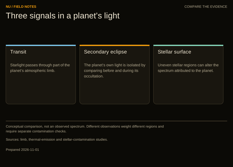
Conceptual comparison, not an observed spectrum. Different observations weight different regions and require separate contamination checks.
A planet's outline is becoming a measurement
On 14 October 2026, a Nature Astronomy paper reported a spatially varying view of the atmospheric limb of WASP-17 b. Its transmission-strings analysis used JWST observations to infer differences around the planet's silhouette rather than reducing its atmosphere to one uniform ring. The observations themselves were obtained in March 2023. The result is a reconstruction from changing starlight, not a resolved photograph of clouds surrounding the planet. A spatial map of the atmospheric limb of a hot Jupiter.
That distinction captures an important change in exoplanet science. A distant atmosphere was once commonly introduced as a list of molecules identified from characteristic spectral features. Molecular identification remains central, but the measured spectrum also depends on where the light traveled, which part of the star illuminated the atmosphere, and how different regions of the planet were combined. A gas can be present without leaving an observable feature. A feature can be real without uniquely identifying its source.
The practical object is a time series: detector measurements taken while the geometry changes. Before transit, the telescope receives the unobscured star and any unresolved planetary contribution. During transit, the planet blocks part of the stellar disk, while a much smaller component of the light passes along atmospheric paths. During an eclipse behind the star, the planet's own contribution disappears from view. Each arrangement asks a different physical question.
Following those questions is more useful than treating every new spectral bump as another item on a cosmic shopping list. It explains why a hot giant can yield a detailed chemical result while a small temperate planet remains ambiguous. It also explains why observations that appear less spectacular—a second visit, a comparison planet, a different wavelength range—can change an atmospheric interpretation more than another elaborate model applied to the original data.
What a transit spectrum actually measures
For a uniform stellar disk and an opaque circular planet, the fractional loss of light is the projected area ratio: the planet's radius divided by the star's radius, squared. A real transit requires additional treatment of the star's brightness pattern and the planet's trajectory. The elementary area relation nevertheless explains why atmospheric spectroscopy works: wavelength-dependent opacity changes the effective blocking radius.
Timothy Brown's foundational transmission calculation described this observable as a ratio of in-transit and out-of-transit spectra. In that model, atmospheric composition, temperature, clouds and winds alter the wavelength-dependent outline through which tangential rays can pass. Its importance is the forward relationship between physical atmosphere and measured light, not an assumption that every spectrum has a unique inverse. Brown, 2001.
Consider an invented geometric example. A planet of radius 10,000 kilometres crosses a uniform star of radius 100,000 kilometres. The opaque disk removes one percent of the starlight. If an absorbing band adds an effective height of 50 kilometres, the extra fractional area is approximately twice the planetary radius times that height, divided by the squared stellar radius. The result is 0.0001, or 100 parts per million. Keeping the same planet but doubling the stellar radius reduces this atmospheric increment to 25 parts per million.
Those numbers are not a prediction for an actual target. They hold the effective atmospheric height fixed and omit limb darkening and other effects. Their purpose is to separate the large broadband transit from the much smaller wavelength-dependent change. Measuring that change requires comparing light curves with a common geometric account, not simply finding a dark line in a conventional photograph.
An effective height is also not a material boundary. At each wavelength, a range of rays encounters different optical depths. The reported transit radius summarizes their combined attenuation. A line drawn around a model planet should therefore not be mistaken for the altitude of a solid surface or a sharply defined cloud top.
A long sideways path through thin gas
An atmospheric ray near the limb passes sideways through gas that would occupy a much shorter column in a vertical view. Transmission can consequently become opaque at pressures where a downward-looking measurement would still see deeper. This geometry makes a thin upper atmosphere important to the observed silhouette and restricts what can be learned about material beneath it.
The relevant vertical length scale can be estimated from hydrostatic balance and the ideal-gas relation. For an isothermal atmosphere with approximately constant gravity, the pressure scale height is Boltzmann's constant times temperature divided by mean molecular mass and gravitational acceleration. Pressure falls by a factor of the mathematical constant e over one such height. The assumptions describe a useful local approximation, not every part of an escaping or strongly structured atmosphere.
For a hypothetical temperature of 600 kelvin, gravity of ten metres per second squared and mean molecular mass of 2.3 atomic mass units, this expression gives a scale height of about 217 kilometres. Replacing the mean molecular mass with 28 atomic mass units, while retaining temperature and gravity, gives about 17.8 kilometres. The difference is roughly a factor of twelve. A small spectral modulation can therefore reflect a compact heavy atmosphere rather than little gas.
A separate geometric estimate makes the sideways effect concrete. For a thin exponential atmosphere, a characteristic slant-to-vertical column enhancement is approximately the square root of twice pi times planetary radius divided by scale height. An invented radius of 10,000 kilometres and scale height of 20 kilometres give an enhancement near 56. This is an idealized tangent-path calculation, not an observed pressure level. Fortney, geometry derivation, 2005.
The physical lesson is selective access. Transmission emphasizes the parts of an atmosphere that remain accessible along long slant paths. An interpretation of deep oceans, surface pressure or lower-atmosphere chemistry needs additional evidence connecting those inaccessible regions to the thin layer that the spectrum samples.
Radius does not arrive with a pressure label
The radius obtained from a transit does not automatically tell an astronomer the atmospheric pressure at that radius. That missing label couples several inferred quantities. A model can sometimes compensate for a different reference pressure by changing an absorber abundance or the assumed reference radius, producing similar spectral structure.
Heng and Kitzmann examined this normalization problem in the context of Hubble's WFC3 transmission spectra. Their analysis connects the reference-radius, reference-pressure and water-abundance ambiguity, and provides analytical descriptions under specified atmospheric assumptions. It does not establish that every wavelength-rich JWST analysis must have exactly the same unresolved degeneracy. Heng and Kitzmann, revised June 2017.
An elementary absorption example shows why an ambiguity can occur. In an optically thin uniform slab, attenuation depends approximately on absorber number density multiplied by cross section and path length. If the cross section and path are known but total gas density is not, doubling the total density while halving the absorber fraction preserves the absorber column. The spectrum may constrain that column better than either of its ingredients separately.
An actual atmosphere is more complicated: lines saturate, collision effects change opacity, temperature varies, and several absorbers overlap. Those complications can add information as well as uncertainty. A feature whose shape depends on pressure can help distinguish cases that would be identical in the simple slab. Broad spectral coverage may supply another independent constraint. Neither improvement should be presumed merely because a fitting program returns narrow intervals.
A useful atmospheric result identifies which combinations the observations really constrain. A molecular feature can be securely associated with a species while its absolute abundance remains less precise. Conversely, an apparently precise abundance can depend strongly on fixing a reference quantity that the data themselves scarcely determine. Reporting those relationships preserves the scientific value of detection without overstating the inventory.
The spectrum begins as a detector problem
A telescope does not directly record a table of transit depths. It records a sequence of detector readouts. Producing a spectrum involves calibration, identifying the spectral trace, estimating background, extracting flux, assigning wavelengths and fitting its temporal variation. Choices made early in this chain can affect later atmospheric conclusions.
The original Eureka! software paper describes an open, modular route from uncalibrated time-series files to transmission or emission spectra. Its publication in November 2022 documents an analysis architecture, not a certification that every reduction using the package is free of systematic error. Bell and colleagues, Eureka!.
Imagine a spectral trace moving slightly across detector pixels whose sensitivities are not perfectly characterized. The star has not changed, but the extracted signal may change. If the motion happens on a timescale similar to ingress or egress, a correction can become correlated with transit shape. An excessively flexible correction may absorb part of the planet signal; an insufficient correction may leave an instrumental pattern that resembles one.
Background subtraction poses a different problem. Suppose a hypothetical wavelength channel contains 100,000 stellar counts and 1,000 background counts in a chosen interval. An error of ten background counts is only one percent of the background but 100 parts per million of the stellar signal. Describing the background as small does not show that its uncertainty is irrelevant to atmospheric spectroscopy.
Independent reductions are valuable when they genuinely vary relevant choices. Two teams using the same calibration products and identical extraction assumptions may share an error even if their software has different names. The informative comparison follows intermediate products: which pixels, integrations or fitted terms produce a disagreement? That makes a disputed feature a tractable measurement question rather than a competition between final colored curves.
Binning trades detail for precision
A spectrum is commonly displayed in wavelength bins, each combining measurements over a finite interval. Larger bins collect more photons and can reduce independent noise, but they merge nearby structure. Smaller bins preserve shape while leaving less information in each point. Neither choice creates a universally better spectrum.
In a deliberately simple example, four independent channels each have equal uncertainty of 80 parts per million. Their equally weighted average has uncertainty of 40 parts per million. But if they all share an additional wavelength-correlated error, that common contribution does not shrink by the same factor. Displaying fewer, smoother points can conceal that distinction.
The location of bin edges matters when a feature is narrow or when neighboring measurements are correlated. A peak split between two bins may look less striking than the same signal centered in one. This is not evidence of misconduct or proof that the feature is false. It is a reason to test whether the physical conclusion survives reasonable representations of the same underlying measurements.
Spectral resolving power introduces a related limit. Defined as wavelength divided by the smallest distinguishable wavelength interval, it describes how finely an instrument can separate structure. At four micrometres, a hypothetical resolving power of one hundred corresponds to an interval of about 0.04 micrometres. Plotting samples at much closer spacing does not necessarily provide independent physical resolution.
These considerations change observing strategy. A broad isolated band may benefit most from precise low-resolution coverage. Several overlapping species may require resolving their different internal patterns. The choice should be tied to the alternatives being distinguished. More points, smaller error bars and a more visually intricate plot are not interchangeable forms of information.
Molecular fingerprints require a physical library
Molecules absorb through transitions between allowed energy states. Their spectral patterns depend on temperature, pressure and the surrounding collision partners, not just their names. A model needs line positions and strengths, and an account of how individual lines combine after atmospheric and instrumental broadening.
The 2024 ExoMol database paper describes molecular line lists and associated products for hot-atmosphere spectroscopy, including attention to accurate energy levels and collisional broadening. Such databases supply part of the physical translation between a chemical hypothesis and a predicted spectrum. The article's calculations do not become independent of laboratory or theoretical molecular data simply because the astronomical observations are new. Tennyson and colleagues, ExoMol 2024.
Consider a hypothetical pair of molecules that both absorb near one broad wavelength region. If one also produces a second band within the observed range while the other does not, that second region can be more decisive than a slightly better fit to the shared band. If the second band lies outside the instrument's coverage, the inference remains less discriminating. Missing spectral coverage is not equivalent to observing the band and finding it absent.
Temperature can further alter the comparison by changing the populations of molecular energy states. A room-temperature absorption template may omit transitions that matter in a much hotter gas. Conversely, adding every imaginable molecule without credible opacity data does not create a complete alternative model. The quality and applicability of the molecular library are part of the uncertainty budget.
This is why a feature is better understood as a pattern of constraints than a barcode read in isolation. Positions, relative strengths, wavelength coverage and physically plausible conditions work together. The strongest identification is the one whose predicted structure survives independent opportunities to fail, rather than the one whose name most readily matches a single broad bump.
The illuminating star is not a uniform lamp
The light blocked during a transit comes from the narrow strip crossed by the planet. The comparison light comes from the entire visible stellar disk. If those regions have different spectra, dividing in-transit by out-of-transit light does not perfectly cancel the star. Cooler spots and brighter surface regions can leave wavelength-dependent signatures in the apparent planetary spectrum even when the planet never crosses them.
Rackham, Apai and Giampapa modeled this transit light-source effect and showed that rotational brightness variability does not uniquely determine the surface covering fractions needed to predict contamination. A weakly varying light curve is therefore not, by itself, a certificate of a spectrally uniform star. The transit light-source effect, revised January 2018.
Here is an idealized calculation, deliberately excluding limb darkening. Let a planet block one percent of an unspotted region's brightness. If unocculted spots lower the star's disk-averaged brightness to 98 percent of that reference, the apparent transit depth becomes 0.01 divided by 0.98, or about 0.010204. That is roughly 204 parts per million deeper than the uncontaminated one-percent transit. If the stellar contrast changes with wavelength, the apparent change is spectral rather than a single constant offset.
The example does not estimate any real star's spot coverage. It demonstrates why contamination is multiplicative: the denominator of the measurement has changed. Subtracting an arbitrary smooth curve afterward is not always equivalent to modeling the illuminating geometry.
An observed warning, not just a theoretical nuisance
JWST observations of TRAPPIST-1 b supplied an empirical example of this problem. Lim and colleagues reported two NIRISS visits with different contamination patterns associated with unocculted stellar heterogeneity. Their analysis retained a constraint against cloud-free hydrogen-rich atmospheres while not establishing whether a secondary atmosphere was present. This is a case where an atmospheric exclusion and substantial stellar ambiguity coexist. Lim and colleagues, September 2023.
Those statements are not contradictory. An observation may reject a class of large predicted features while remaining unable to discriminate among smaller alternatives. Rejecting a transparent, extended hydrogen atmosphere does not reject every possible layer of gas. Nor does recognizing a stellar contaminant mean that every planetary constraint disappears.
For a hypothetical observing campaign, imagine that the expected planetary feature is stable across visits but the star's contribution changes. Fitting all visits with one planet spectrum and separate stellar terms can exploit that difference. Yet a persistent stellar feature could also remain stable. Repetition tests temporal variability; it does not automatically identify the origin of everything that repeats.
The choice of a common planet spectrum is itself conditional. Atmospheric weather can change, especially on strongly irradiated worlds. A method that forces all genuine planetary variation into stellar nuisance terms could become misleading in another regime. The relevant timescales and expected amplitudes need physical justification rather than a blanket rule that planets are constant and stars are variable.
An observing log consequently carries scientific information. Stellar activity indicators, flare timing, detector behavior and the placement of the transit within the visit can help distinguish explanations. Keeping those records visible makes a spectrum more than a set of averaged points and gives later investigators a way to reconsider the separation.
A neighboring planet can serve as a control
A program described by Allen and colleagues in December 2025 uses closely spaced transits of TRAPPIST-1 e and b to investigate stellar contamination. The approach treats b as an effectively airless comparison object for this purpose. Its first observations show both the promise of transferring stellar information between transits and sensitivity to flares and reduction choices; they are not a detection of an Earth-like atmosphere on e. JWST TRAPPIST-1 e/b program.
The underlying experimental move is elegant: observe a second object that samples the troublesome light source, rather than asking a single spectrum to determine both source and atmosphere. But a control is useful only to the extent that its relevant conditions match. Different transit paths can cross different surface regions. The star can change between the events. Any wavelength-dependent signal intrinsic to the comparison planet would also enter the correction.
A ratio additionally carries the uncertainty of both measurements. If two independent quantities each have a one-percent fractional uncertainty, their ratio has approximately a 1.4-percent fractional uncertainty in the small-error limit. That invented example shows the price of the control measurement. Removing a bias can improve an inference even while increasing the formal random error.
The appropriate test is therefore not merely whether the corrected spectrum looks flatter. One should ask whether injected planetary structure survives the correction, whether the inferred stellar behavior agrees with other observations, and whether the uncertainties include the comparison measurement. A flatter result might represent successful contamination removal or accidental removal of information.
This is a recurring advantage of purposeful observing design. The additional exposure is chosen to distinguish causes, not merely to extend the same time series. A well-matched control can add a kind of information that many repeated measurements of the original configuration cannot provide.
Testing what the analysis would recover
A September 2026 author manuscript by Rathcke and Buchhave develops an empirically calibrated atmospheric-search framework for TRAPPIST-1 c. It uses multiple epochs and injection-recovery tests, with archival observations of b as a control for contamination. The methodological contribution is to test recovery against real troublesome data rather than relying only on idealized white-noise simulations. Rathcke and Buchhave, version 1.
An injection test adds a known artificial signal and asks whether the analysis finds it. Its interpretation depends on where the signal enters. Adding a molecular pattern to an already extracted spectrum tests the subsequent retrieval. Adding an appropriate signal earlier in a simulated detector sequence can test more of the reduction chain. Neither test automatically validates stages that the injection bypasses.
Suppose, as an illustrative exercise, one hundred synthetic features of a particular amplitude are placed in independent trial datasets, and eighty are recovered under a prespecified rule. That estimates recovery behavior for that amplitude, feature shape and dataset construction. It does not show that an observed feature has an eighty-percent chance of being real. Recovery and false-positive behavior answer different questions.
A second set of trials with no added planetary signal can investigate spurious detections. Varying the injected temperature, cloud structure or molecular mixture tests whether success depends on an overly convenient template. A method that recovers only the exact model it was designed around may perform poorly when the actual atmosphere departs from that family.
The outcome can guide telescope time more intelligently than a simple square-root exposure forecast. If a feature disappears into a persistent stellar pattern, collecting more of the same configuration may have limited value. A different comparison, wavelength range or stellar constraint may be the experiment that changes the answer.
Clouds can conceal gas without removing it
A cloud or haze can truncate the range of paths through which gas is visible. In transmission, a high opaque layer can prevent rays from reaching deeper material. The resulting muted molecular features do not necessarily imply low molecular abundance. A compact atmosphere and an obscuring aerosol layer can produce related observational consequences through different physics.
An original toy model clarifies the distinction. Imagine a gas whose absorption band becomes opaque five scale heights above a reference level while the nearby continuum becomes opaque one scale height above it. The spectral height difference is four scale heights. Add a completely opaque, wavelength-independent cloud top at three scale heights. In this simplified construction, the continuum now starts at three while the band still reaches five, leaving only two scale heights of contrast. The gas abundance has not changed.
Real aerosol opacity is not necessarily gray. Particle composition, size and shape can produce slopes or absorption structure. A model that represents every cloud by a flat barrier can be useful for some data but inappropriate when the observations resolve those properties. Conversely, fitting many aerosol parameters to a featureless spectrum may return freedom rather than a measurement.
Partial cloud cover adds another complication. An observed limb can combine clear and cloudy sectors. Their transmitted fluxes are averaged before being translated into an effective radius, so the result need not equal the spectrum of a uniformly cloudy atmosphere with the average cloud pressure. The same issue appears whenever different regions contribute nonlinearly. Line and Parmentier, non-uniform cloud models, revised February 2016.
A meaningful nondetection therefore names the excluded atmospheres. It might rule out a specified clear, low-molecular-mass model while remaining compatible with a cloud-covered alternative. The distinction is not verbal caution layered onto an otherwise complete answer. It is the actual physical content of the measurement.
Why averaging two atmospheres can invent a third
One-dimensional retrievals are computationally attractive because they describe an atmosphere using a single vertical column. But a transit combines different locations. If morning and evening differ in temperature or chemical composition, the combined spectrum can resemble a one-dimensional column that exists nowhere on the planet.
MacDonald, Goyal and Lewis demonstrated this with synthetic spectra and retrievals: applying a single-column model to atmospheres with different morning and evening compositions can bias recovered temperatures and abundances even when the fitted spectrum looks acceptable. The finding is about model mismatch in the tested configurations, not a claim that all one-dimensional atmospheric analyses are invalid. MacDonald and colleagues, 2020.
The mathematical issue can be illustrated without a planet model. Transmission through an absorbing path is proportional to the exponential of negative optical depth. Suppose half the contributing area has optical depth zero and half has optical depth two. The average transmitted fraction is about 0.568. A single path with the average optical depth of one transmits only about 0.368. Averaging conditions before calculating transmission is not the same as calculating transmission before averaging.
A retrieval trying to fit the first number with the second kind of model must change something: abundance, temperature, geometry or a cloud parameter. Those adjustments can make the predicted spectrum agree while moving the inferred atmosphere away from the actual regional conditions.
Ingress and egress provide one route to additional spatial information because the star covers different parts of the projected planet at different times. But the gain comes with stronger demands on timing, stellar brightness and instrumental stability. A reconstructed limb map inherits those dependencies. Its scientific value lies in testing spatial alternatives, not in making an unresolved planet resemble an ordinary photograph.
Emission opens a different atmospheric window
A secondary eclipse measures the disappearance of the planet's contribution when it passes behind the star. In the infrared that contribution can include thermal radiation. Comparing the combined light just outside eclipse with the star alone during eclipse provides a planet-to-star flux ratio, subject to temporal and instrumental modeling.
A 2024 JWST study of the rocky planet 55 Cancri e used NIRCam and MIRI thermal-emission measurements to argue for a substantial volatile atmosphere rather than the tested tenuous rock-vapor scenario. The authors favored carbon-bearing atmospheric possibilities. This is evidence about a very hot planet under specified models, not evidence for a temperate surface or inhabited environment. Hu and colleagues, May 2024.
Emission and transmission should not be compared as though they sample the same column. During eclipse, the visible dayside contributes a projected-disk average. During transit, starlight probes long paths near the boundary between day and night. Different pressures and temperatures can dominate each observable. Apparent disagreement may therefore reveal atmospheric structure rather than a failed measurement.
Thermal features also depend on the vertical temperature profile. Increasing opacity at one wavelength changes the heights from which radiation escapes. If those heights are cooler than the surrounding continuum-forming region, a band can appear in absorption. With a suitable temperature inversion, the same species can produce emission structure. Identifying the gas and inferring the temperature profile are linked tasks.
A brightness temperature is the temperature of a blackbody that would produce the measured radiance at a specified wavelength. It is not automatically the temperature of a solid surface or the average temperature of the entire atmosphere. Combining several brightness temperatures into a physical profile requires the opacity and geometry that determine which layers the measurement weights.
An orbit provides changing views, not independent photographs
A phase curve follows the unresolved planet as different portions of its illuminated and dark hemispheres face the observer. Its wavelength dependence can help distinguish thermal contrasts, transport and opacity. The observations remain disk-integrated: a point on the curve combines many locations, weighted by viewing geometry and emission.
Bell and colleagues reported a phase-resolved JWST/MIRI spectrum of WASP-43 b in 2024. Their analysis and comparisons with three-dimensional models supported a large day-night contrast and nightside clouds, with water absorption across the observed phases. The interpretation uses both temporal behavior and spectra; it is not a direct cloud image. Bell and colleagues, WASP-43 b.
A displaced brightness maximum can provide evidence about how the brightest region relates to the substellar direction, but converting that offset into a wind speed requires a model. Radiative cooling, circulation, clouds and the pressure level being observed all affect the relationship. Two bands can peak at different phases because they weight different atmospheric layers rather than because one measurement is wrong.
There is an inverse-problem limit as well. A small bright patch and a larger moderately bright region can contribute similar total flux. Some spatial patterns largely cancel when integrated over the visible disk. A reconstruction that shows many fine regions may be displaying the model's permitted detail more than the data's independent information.
The productive approach is to ask which spatial distinctions change the observable. Does a proposed cloud pattern predict the right spectrum as well as the right phase amplitude? Does a circulation model account for several wavelength bands without changing its basic physics between them? Those cross-constraints are more informative than assigning a meteorological label to one fitted offset.
Chemistry is a network operating out of equilibrium
A retrieved molecular abundance is an atmospheric state, not an explanation for how that state arose. Chemical equilibrium calculations predict a composition for specified conditions, but irradiation and transport can drive an atmosphere away from those local expectations. Molecules can be produced aloft, destroyed by photons or carried between regions faster than reactions restore equilibrium.
For WASP-39 b, Tsai and colleagues used photochemical models to explain a sulfur-dioxide feature associated with JWST observations. Their work links the spectral interpretation to a reaction network driven by stellar irradiation. This is an example of chemistry providing a physical account of an observed absorber, not merely adding another free abundance to a fit. Photochemically produced sulfur dioxide, revised March 2023.
The competition can be expressed with timescales. If vertical transport moves material through a region in a hypothetical ten thousand seconds while the relevant chemical adjustment requires a million seconds, local equilibrium is unlikely to be restored during that passage. Reversing those timescales changes the expectation. The actual rates must be calculated for the relevant reaction network, pressure and temperature; the example supplies no estimate for a named planet.
The host star matters here in a second way. Its surface spectrum can contaminate the observation, while its irradiation physically changes the planet's atmosphere. Those are separate effects. Correcting a stellar contribution in the measured spectrum does not remove the need to understand the radiation that drives atmospheric chemistry.
A chemically plausible explanation is stronger when it predicts more than the feature that motivated it. Associated species, altitude dependence or responses to temperature can offer additional tests. Failure to observe every predicted companion is not immediately decisive, because observability differs, but the forward calculation should state where the proposed chemical network could be challenged.
Identification, abundance and environment are different claims
The early JWST carbon-dioxide result for WASP-39 b illustrates a comparatively clear molecular identification: the reported spectrum included a prominent band near 4.3 micrometres, supported by atmospheric modeling. The observation established a spectral association in a hot gas giant. It did not make carbon dioxide a unique marker of any particular surface environment. JWST Early Release Science team, August 2022 manuscript.
Three questions should remain separate. Is an absorber needed to explain the data? What range of abundance is compatible with the atmosphere and reference assumptions? What environments can produce that abundance? Progress on the first does not automatically solve the second, and neither necessarily singles out one answer to the third.
A hypothetical pair of atmospheres might both contain the same detectable gas but differ in bulk composition, temperature and deep boundary conditions. One may yield a large transmission feature because the atmosphere is extended; another may contain more of the gas but present a smaller observable modulation because the mean molecular mass is higher. Ranking feature heights is not the same as ranking concentrations.
Even elemental abundance ratios require care. A measured molecule contains only part of an element's atmospheric inventory. Unobserved molecules, condensates or deeper reservoirs may hold the rest. Inferring a bulk carbon-to-oxygen ratio from a limited set of absorbers therefore introduces chemical and structural assumptions beyond identifying those absorbers themselves.
This layered interpretation makes comparison across planets more useful. Rather than placing every published abundance into one undifferentiated table, researchers can compare results obtained with compatible wavelength coverage, pressure sensitivity and model flexibility. The goal is to find real planetary diversity without accidentally classifying differences between observing methods as differences between worlds.
A contested molecule is not an established biosphere
The K2-18 b debate provides a concrete warning about moving too quickly through those layers. An April 2025 paper reported evidence favoring dimethyl sulfide and/or dimethyl disulfide in a JWST mid-infrared spectrum, while calling for further observations and better chemical information. That is the authors' interpretation of their analysis, not a confirmed biological finding. Madhusudhan and colleagues, April 2025.
A subsequent joint analysis by Luque and colleagues examined near- and mid-infrared observations with multiple reductions and retrieval approaches. It found insufficient evidence for those molecules and showed that alternative molecular choices could fit the relevant structure. This dated comparison demonstrates sensitivity to the data treatment and competing absorbers; it should not be turned into a claim that every future K2-18 b observation has already been decided. Luque and colleagues, May 2025 manuscript.
The first task is to establish what the spectrum requires. Only afterward does the origin of a confidently identified gas become the central question. A compound associated with organisms on Earth can have different sources or sinks under another planet's temperature, irradiation and chemical environment. An abundance that seems surprising under one abiotic model does not exhaust the space of nonbiological explanations.
Nor does an atmosphere compatible with an ocean prove that an ocean exists. Interior structure, atmospheric mass, temperature profiles and the coupling between deep reservoirs and the observable atmosphere must be constrained. Several physically different planets can occupy overlapping regions of mass, radius and atmospheric parameter space.
The appropriate conclusion is not that atmospheric searches for life are pointless. It is that they require a chain of independently testable arguments. A spectral feature, a molecular identification, an environmental model and a biological interpretation are distinct links. Telescope sensitivity can strengthen the first link while leaving another as the weakest part of the chain.
Choosing the next observation by its disagreement
Suppose two plausible models fit the existing spectrum but make different predictions outside its wavelength range. The most useful next exposure may target that disagreement rather than repeat the strongest existing band. If the models differ mainly in their response to stellar contamination, a comparison transit or monitoring of the host could be more valuable than extending planetary coverage.
An explicit planning example makes this concrete. Imagine models A and B that differ by 100 parts per million in one band and only ten in another. If an observation could achieve equal, independent 25-part-per-million uncertainties in both, the first band has much greater discriminating potential. But if that band is dominated by a poorly characterized stellar feature, its apparent advantage can disappear. The measurement plan must include the nuisance physics, not just the separation of ideal curves.
Temporal placement also matters. Enough baseline before and after an event helps constrain slow trends. Ingress and egress support geometric inference. Repeated visits test stability. These are different uses of observing time, and the preferred allocation depends on which ambiguity limits the current result.
A useful published spectrum leaves that decision open to others. It provides the time series or accessible data products, calibration choices, covariance information, model assumptions and enough detail to reproduce the comparison. A figure with tiny error bars is less informative when the correlations and discarded intervals are inaccessible.
The emerging achievement is not a catalogue in which every distant world receives a definitive atmospheric label. It is a set of experiments increasingly able to distinguish physical explanations for very small changes in light. The most revealing result may be a molecule, a spatial contrast or an exclusion. Its strength comes from knowing which part of the atmosphere—and which part of the measurement—has actually been brought into view.